motion and time based algorithmic modelling in architectural design: mathematical curves in the effect of natural phenomena
This English version is a direct machine-assisted translation of the Turkish page and will be revised. The Turkish original is authoritative.
Against the conventional disciplinary perspective’s approach of placing the end product at the centre, this research examines design’s capacity to construct and manage a process. Through the real-time data of a sphere object moving in nature, it reveals the mathematical curves formed under the influence of external forces such as gravity and wind, and the information-bearing surface variations that these curves generate on the topological plane. Structured through the stages of concept, experiment, observation and model, the study offers, instead of a fixed form, an open-source design process model that can adapt to any situation.
thesis process and jury dates
- Aug 2014start of doctorate
- May–Jun 2016thesis proposal · Interdisciplinary Research and Development Studies in Parametric Design and Research Pavilion Design
- Dec 2016thesis monitoring committee 1 · The Problem of Morphology in Architecture: A Study of Parametric Structure Design
- Jun 2017thesis monitoring committee 2
- Dec 2017thesis monitoring committee 3 · title proposals on architectonic language
- Dec 2018thesis monitoring committee 4 · tectonic evolution
- Jun 2019thesis monitoring committee 5 · morphology, performance, catenary curve
- Jan 2020jury report · motion capture and mathematical curves; the present direction of the thesis
- Oct 2020thesis monitoring committee · first report under the new title · Motion and Time Based Algorithmic Modelling in Architectural Design
- Mar 2021thesis monitoring committee
- 25 Jun 2021thesis monitoring committee
- Dec 2021thesis monitoring committee
- 24 Jun 2022thesis defence (online) · unanimous decision for revision
- Dec 2022revision defence
- 18 Apr 2023thesis approval
defence jury and supervisors
- Prof. Dr. Sercan Özgencil Yıldırım (supervisor)
- Prof. Dr. Levent Arıdağ (co-supervisor)
- Prof. Dr. Fitnat Cimşit Koş
- Assoc. Prof. Dr. Mustafa Orkun Özüer (Beykent University)
- Prof. Dr. Hakan Sağlam (Ondokuz Mayıs University)
- Assist. Prof. Dr. Zülal Nurdan Korur (Istanbul Medipol University)
thesis monitoring committee
- Prof. Dr. Sercan Özgencil Yıldırım (supervisor)
- Prof. Dr. Levent Arıdağ
- Prof. Dr. Fitnat Cimşit Koş (from the 4th thesis monitoring committee onwards)
- Assoc. Prof. Dr. Mustafa Orkun Özüer
- Prof. Dr. Salih Ofluoğlu (thesis monitoring committees 1–3)
- Prof. Dr. Yavuz Koşaner (qualifying examination jury)
experimental research framework and methodology
concept · experiment · observation · model
The transformation of time from a cyclical order into an absolute line, and from there into the space-time continuum; with Greg Lynn, time becoming a design parameter that generates form. Physical models in which forces find form, the continuity of topology, and the blob as an information-bearing surface interacting with external forces.
How motion is represented: Muybridge’s sequential series and Marey’s time superimposed in a single frame. With chronophotography carried onto the time plane, the trace of motion turning into a curve along linear, circular and Möbius trajectories.
The trace of natural phenomena in the motion of the sphere as a geometric body: weight changing the apex, wind changing the rhythm. Real-time data being written into the curve as information, and the trajectory and the distance between photographs becoming design parameters.
Not an object but a design process model: the transition from the sphere to the blob fusing through fields of interaction. The distance between the spheres and the material density determine the smoothness of the surface; instead of a single final form, ten variations of information-bearing surfaces.
conceptual framework: time, force and the evolution of form
This chapter takes form generation in the discipline of architecture out of static coordinate systems and redefines it through the relations of time, motion and force. Starting from philosophical and physical readings of time, it lays the foundations for the search for dynamic form in the balance of natural forces and in the computational design environment.
readings of time and motion: from plato to einstein
The transformation of time into a parameter in design practice is directly linked to the philosophical and physical transformation of the time–motion relationship over the course of history:
In the Timaeus dialogue, Plato places the regular motion of the planets and the fixed stars at the centre of the creation of time. Time is defined by the countable, recurring and cyclical motions of the celestial bodies. For Plato, disorder is a metaphysical realm; time, by contrast, is not a linear segment bounded at both ends but a circular line closing back on itself in an endless cycle. This understanding accepts the existence of motion as the precondition of time (Thein, 2021; Vázquez, 2022: 119).
In the texts of Physics IV (10-14), he constructs time directly through the concept of "change". Time is the number of motion counted with respect to before and after. For Aristotle, the "now" is like a point on a geometric line; it has no extension or duration. It both forms a definite boundary between past and future and connects them to one another. While change can speed up and slow down, time is constant; time is therefore not change itself but the regulating limit within the flow of motion (Coope, 2005: 34–35, 91–95; Falcon, 2013: 49–50).
With the Principia (1687), he separates time completely from sensory perceptions and physical changes. Unlike relative and sensible time, "absolute and mathematical time" flows uniformly by its own nature, without relation to any external object or force. Unlike in Aristotle, time here is prior; motion becomes a function of time as an independent mathematical variable. All physical quantities such as velocity, acceleration, momentum and force are defined on this absolute timeline (Motte, 1846: 77–78; Turetzky, 1998: 76–78; Toulmin, 1959).
With the theory of relativity, he overturns Newton’s assumption of "an absolute time that is the same for everyone". The flow of time changes according to the observer’s state of motion and frame of reference. Rather than treating three-dimensional Cartesian Euclidean space and linear time as independent variables, Einstein adds time (t) to the spatial coordinates (x, y, z) and establishes the four-dimensional "space-time" (Minkowski space) continuum. In architecture, form is no longer defined as a static sequence of coordinates but as a dynamic state that deforms continuously within space-time (Einstein, 1920a: 30–32, 65; Einstein, 1920b: 8–10).
animation technique in architecture and greg lynn
Greg Lynn abandons the traditional static coordinate plane of architecture (neutral Euclidean space) and reconstitutes the design field as a medium for the active interaction of forces and motion. In line with Lynn’s Animate Form (1999) and Calculus-Based Form approach, animation is not merely a tool for representing motion but a process of form generation in which gravity, wind, fluidity and temporal vectors are defined as force fields in virtual space (Lynn, 1999a: 9–11, 32).
In this process, whereas architecture throughout history discussed time only in the context of a building’s ageing after construction or of its being experienced, Lynn makes time the "constitutive parameter of the design process" in which form is directly conceptualised, develops and grows. Form is no longer a fixed set of coordinates but a state of continuous differential change dependent on time. External factors such as temperature, gravity, wind flows and densities are set up in the design environment as numerical vector fields that deform the form. This deformation is not structural damage; it is the topological transformation that form undergoes as it adapts to changing inputs (Lynn, 1993: 12; Lynn, 1999a: 25).
the relationship and synthesis of the five theoretical ideas in the thesis
Within the scope of the thesis, these five lines of thought are treated not as a linear historical sequence but as a complementary methodological framework. Plato’s circular conception of time becomes operational in the periodic rhythm of the motion the ball traces in the air and in the closed topological continuity of the Möbius strip; Aristotle’s view, which reduces time to the limits of change, finds its counterpart in the division of motion into "now" sections frozen by chronophotographic records. Newton’s independent timeline and mechanics of motion establish that the parabolic traces the ball draws in space are not random but mathematical curves fully calculable through gravity and mass forces. Einstein’s four-dimensional space-time continuum, which unites Euclidean space with the dimension of time, enables the successive photographic moments to go beyond Cartesian limits and form a topological trajectory. All this philosophical and physical groundwork, combined with Greg Lynn’s animation technique and isomorphic surface (blob) theory, moves away from the goal of a final product; it turns into an open-source design process model that deforms, stretches and generates information instantaneously with the real-time forces of natural phenomena.
the balance of forces and physical form-finding
Every object moving in space takes up a position within its own temporality under the influence of internal and external forces. From Gothic vaults onwards, structural force and form have been thought together; Antoni Gaudí (the hanging-string model of the Sagrada Familia) and Frei Otto (soap-film experiments and the Munich Olympic Stadium) searched for the optimal form by simulating natural phenomena such as gravity and surface tension in a physical environment. These approaches are pioneering models that read forces as physical data and turn them into design parameters (Lynn, 2005; Burry, 2016; Özgencil Yıldırım, 2017: 78).
topological transformation and elastic strip trajectories
Topology studies the qualitative relationships that are preserved even when shape and size undergo deformation (Burry and Burry, 2010: 157; Emmer, 2016). Within the research, the time plane was constructed through a three-stage topological transformation based on the geometry of an "elastic strip":
- (1) Linear Trajectory: Placement of the strip on an open, planar axis.
- (2) Circular Trajectory: A radial loop obtained by stretching the strip and joining its ends.
- (3) Möbius Strip: A single-sided topological continuity, formed by turning the strip once around its own axis and joining it, which eliminates the distinction between inside and outside.
isomorphic surfaces (blob / metaball)
When isolated from external forces, the sphere object, a Platonic solid, is a static geometry; when it interacts with neighbouring forces, it turns into a droplet (isomorphic surface / blob / metaball) that stores information and emits a field of influence. Without physically touching one another, blobs fuse through the intersection of their fields of influence, bend, flow towards one another and produce a flexible meta-topology that continually reorganises itself according to instantaneous changes of force (Lynn, 1998: 171–172; Lynn, 1999a: 30).
In isomorphic surface modelling, each sphere defines a field of influence that decreases outwards from its centre. When the interaction fields of two or more blobs overlap, the system mathematically sums the density values of these fields. At a certain threshold value, the surface boundaries are recalculated and a fluid, continuous topological fusion between the spheres is achieved (Kolarevic, 2003: 42).
movement: ball movement
The focus of the research is the motion of the ball; the motion of the body is outside its scope. The temporal displacement of the ball is shaped by the dynamic balance of the pushing force from the hand, air friction, wind and gravity. Since the friction force acts vectorially opposite to the direction of the push, it is included in the model within the push component.
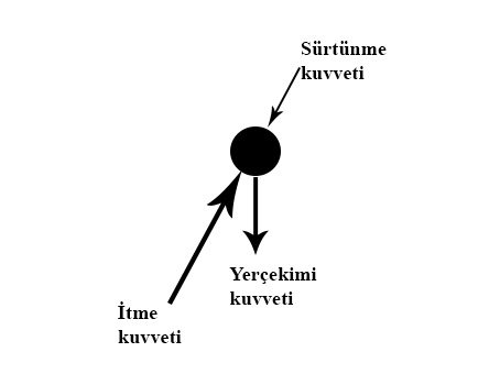 Forces Acting on the Motion of the Ball
Initially the pushing force is greater than gravity and the ball rises along the y-axis. At the apex, the pushing and gravitational forces become vectorially equal and the vertical velocity drops to zero. Gravity then prevails and directs the ball onto its descending path. This process produces a calculable mathematical parabola.
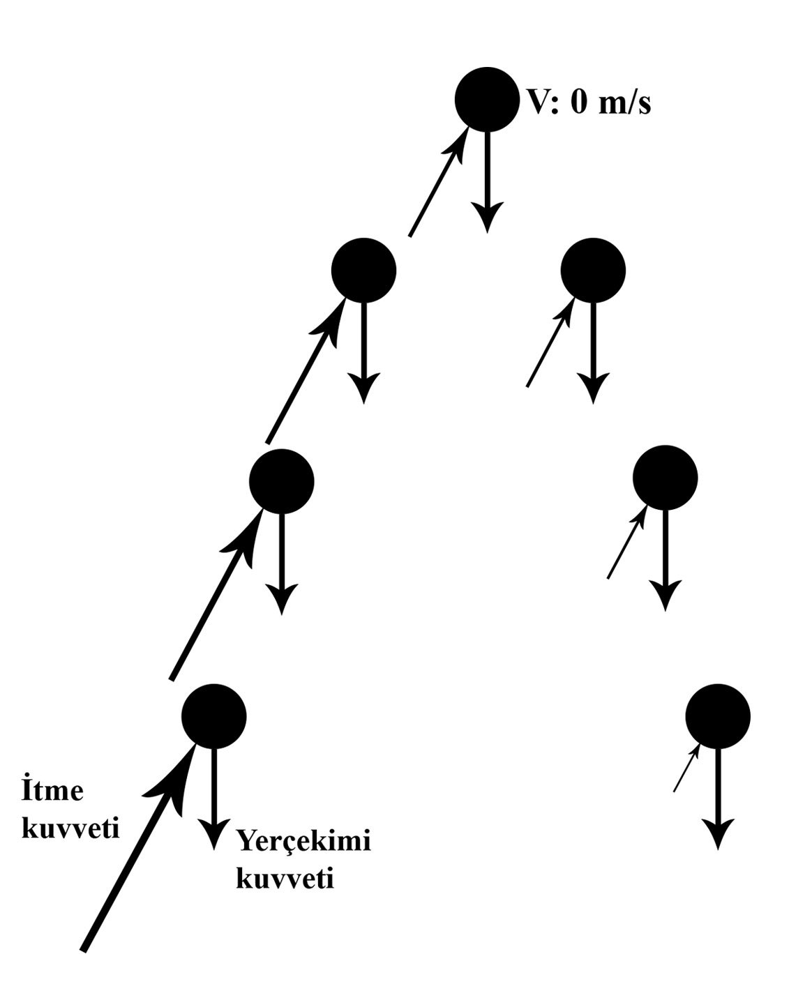 Forces Acting on the Motion of the Ball
To record this motion systematically, the discipline of juggling was drawn upon. The height of the ball under gravity is directly related to the time it stays in the air. To represent this rhythm numerically, the Siteswap mathematical notation language, first introduced by Paul Klimek (1981) and developed in 1985 by groups at Caltech and Cambridge, is used (Buhler et al., 1994; Beek and Lewbel, 1995).
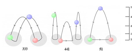 Siteswap Notation (Source: maths.ox.ac.uk/outreach/oxford-mathematics-alphabet/j-juggling)
The notation expresses the time-dependent positions of the balls with numbers. Odd numbers indicate that the ball changes hands, even numbers that it returns to the same hand. In the research model, two basic movement sequences were analysed comparatively: the basic movement 333 (cascade) and the alternative asymmetric movement 423.
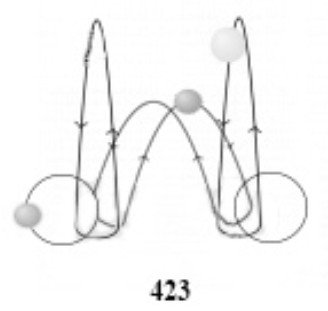 Alternative Movement - 423
experiment: motion capture and form-finding
To transfer motion data from the physical world into the digital environment, 19th-century chronophotography techniques (Muybridge & Marey) were taken as a reference and developed with digital algorithms.
experimental tools: motion capture techniques
According to Vitruvius (80-15 BC), the human body is static in itself and is the source of all geometries. Reinterpreting this view, Leonardo da Vinci (1452-1519) applied, in his sketch 'Vitruvian Man' (1490), a drawing in which the body is not static but standing and in motion. Leonardo da Vinci systematised sixteen possible positions of the human body in the same drawing and, by drawing a circle and a square, showed the body’s relationship with geometry. This dynamism is a primitive representation of the body’s movement. Da Vinci visualised the time/motion relationship (Piedade Ferreira, de Mello and Duarte, 2011).
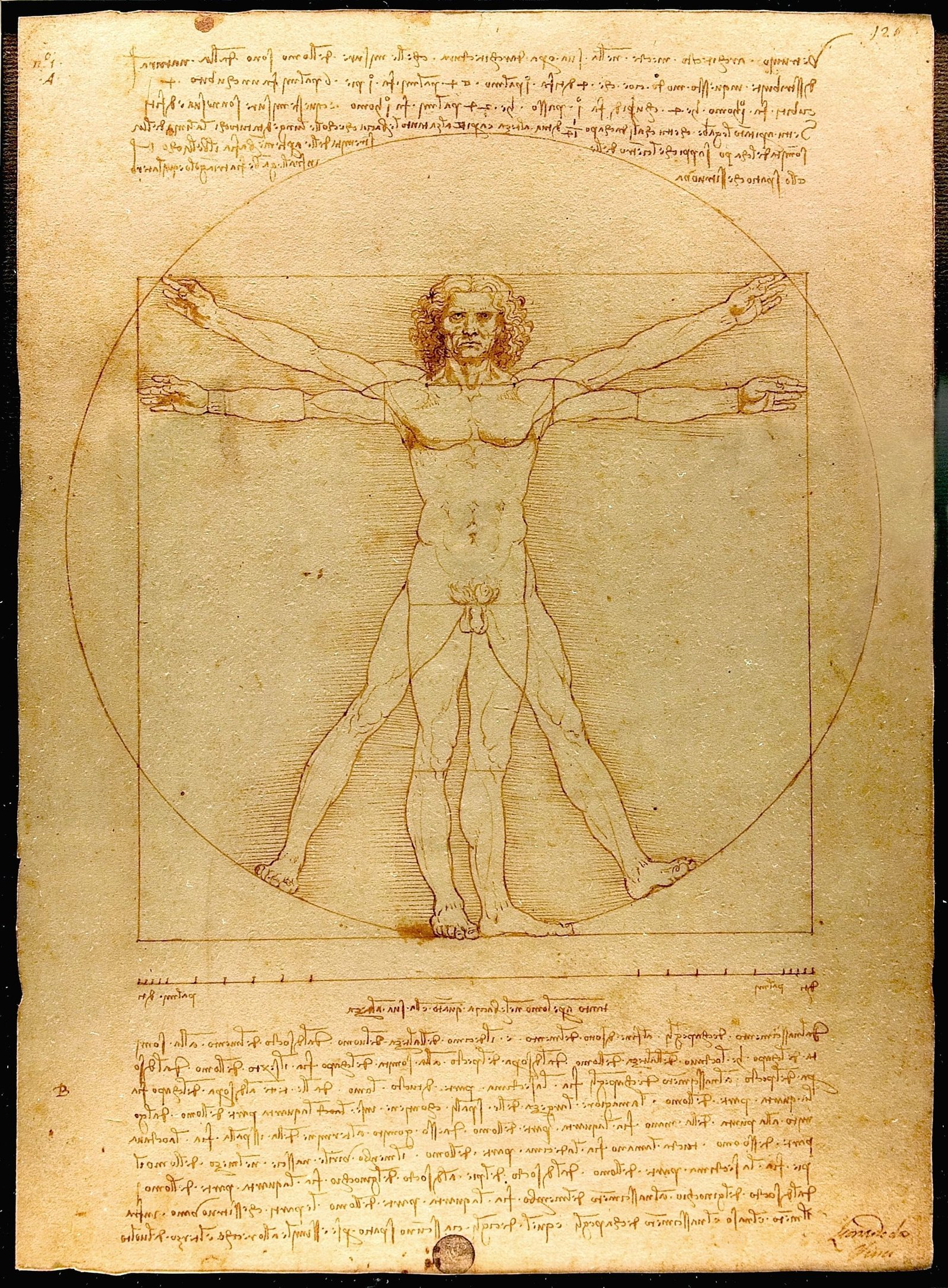 'Vitruvian Man' eskizi (Kaynak: leonardodavinci.net/the-vitruvian-man.jsp)
In the late 19th century, representing time/motion began to be defined as capturing motion. Eadweard Muybridge (1830-1904) and Étienne-Jules Marey (1830-1904) developed a technique, which they called chronophotography, in which they represented motion by taking and composing photographs in a temporal order. Chronophotography formed the basis of the discipline of cinema. As technology advanced, the logical order of chronophotography gave rise to tools such as cameras, phones and motion sensors that can easily capture motion today. In this thesis, the chronophotography technique, the 'Kinect' motion sensor and 'Motion Capture Suit' technology are explained.
The groundwork of the experiments in the research was set up with the chronophotography technique. To understand the software logic of motion capture, experiments were carried out with Kinect and motion capture technology. However, the further development of these sensor-based experiments is planned for post-doctoral work.
chronophotography technique
Chronophotography is the capture of motion over time by taking a series of photographs. Two researchers seeking a method of showing body movement, Étienne-Jules Marey and Eadweard Muybridge, developed the chronophotography technique in the same period in different countries. Both focused on showing body movement graphically, using different techniques. They designed systems for taking a series of instantaneous photographs at very short and equal time intervals, which allowed them to analyse body movements. These systems broke bodily movement down into the smallest possible temporal and spatial fragments within the limits set by the techniques of representation. Muybridge used multiple sequential photographs to show movement. Marey, by contrast, showed movement by combining multiple photographs into a single photograph. With the chronophotography technique, Muybridge and Marey made motion analysis concrete and provided the groundwork for the development of technology.
eadweard muybridge’s chronophotography
The English-American photographic artist Eadweard James Muybridge pioneered motion analysis in California with his photographs of animal and human movement. In the late 1870s, in the debate over whether all four hooves of a running horse touch the ground, he proved the moment at which the hooves do not touch the ground by taking serial photographs of a running horse at equal time intervals. Each recorded frame was captured when the horse stepped on a wire connected to a row of aligned cameras. Although Muybridge had only a series of still images, it is possible to gain an impression of the subject’s movement. In this way, the phases of the movement over a given time interval and the transformation at equal time intervals were observed (Jensenius, 2013).
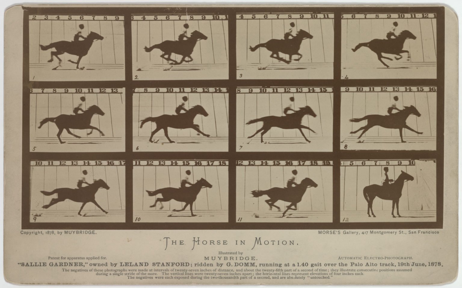 Muybridge’s Running Horse Photograph Series (1878) (Source: smarthistory.org)
Muybridge worked on the visualisation of motion and its becoming a diagram through the chronophotography technique. He developed a clock mechanism so that the cameras he placed in sequence would take photographs with split-second differences. By placing the photographs he took one after another, he discovered the visual representation of motion.
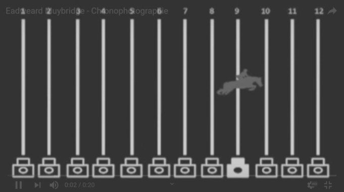 Muybridge’s Serial Photography System
To define the geometric shape of the model, Muybridge created synchronised sequences (separate time frames). He called these the space-time model, otherwise known as the chronoform. It is a model that allows bodies to move forwards or backwards in order to observe their different points in space. The chronoform is the emergence of a series of moments, visualising the narration of a particular event by depicting it through moments ordered in a controlled sequence defined by a geometric path trajectory. This makes the form dynamic while defining the geometry and length of the trajectory path (El Sayary, 2017).
In conclusion, with the emergence of chronophotography, the reflection of time came to the fore. The discipline of photography, with its capacity to record the present moment, refers to Aristotle’s conception of time, which associates time with the motion of objects. Since the photograph records the present moment and thereby forms a boundary between past and future, the 'moment of recording' can be evaluated within the framework of Aristotle’s conception of time, which holds that the arrested present is both a boundary and a connection between past and future. At this point it can be seen that Muybridge, with the chronophotography technique, produced works giving the oscillation diagrams of various models in action, showing every stage of the fragmented motion of an action and its position in space in relation to all the recorded stages.
étienne-jules marey’s chronophotography
Étienne-Jules Marey was a physiologist and photographic artist who lived in France. While researching animal and human movement in the field of medicine, he combined this with the discipline of photography to carry out motion analyses. Like Muybridge, Marey is one of the researchers who laid the groundwork for cinema. In his book "Le Mouvement", Marey wrote that the aim of chronophotography is to determine the characteristics of a movement with precision by representing the different positions in space occupied by moving objects, that is, their trajectory. Although Marey remarked that the mathematical study of his chronophotographic records would be rather complex and of limited interest, he also acknowledged that the motion of certain objects typically produces mathematical forms (Marey, 1984: 24).
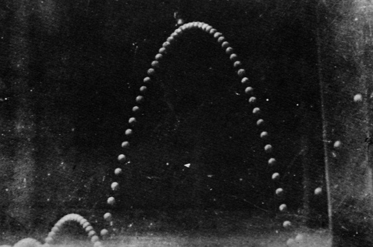 Marey’s Chronophotograph of Ball Motion (1886)
The image above is the chronophotograph in which Marey observed the time/motion relationship of the ball. In this photograph we see that, on the time plane, the distances between the balls decrease as they move away from the ground. However, it was found that Marey had no diagram showing the interval differences of the paired relationships in this photograph. Marey was interested only in the natural curve formed by the trace of the motion and in the paired repetitions of the motion. This chronophotograph guided the experiments carried out in the research. It also prompted the questioning of the paired time/motion relationships together with the natural curve formed by the ball.
Marey realised that the language placed over the image was not verbal but formal. This shows that, in addition to a field of motion and a duration of motion, the understanding of motion is refined by awareness of the emerging form, and that this form, as an independent object of abstract thought, can be extracted from space and real time in order to be worked on. These motion analyses examine the transformations of the body producing the motion and show the balance of forces temporally (Sutil, 2015). Taking Marey’s chronophotography of a flying bird as an example:
 Marey'in 'Bird in Flight' Kronofotografisi (Kaynak: metmuseum.org)
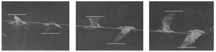 Diagram of Paired Time/Motion Relationships
Looking at the paired relationships in the diagram above, the repetition of the wing movement is observed. However, within the repetition the distance between the wings decreases, and when the bird passes from state 1 to state 3 it has risen relative to state 1. In this case, for the bird to take off, the distance between the wings must decrease. This shows that the balance of the forces acting on the wing transforms according to time/motion. This transformation depends on forces such as air density, wind, friction and gravity, as well as on the wing’s surface area and on the internal structure and form of the wing. As in the ball motion, the paired relationships become integrated with one another. The resulting trace becomes smoother.
Marey was interested in measuring the flow of motion. For this reason, Marey aimed to see the whole of time/motion on a single photographic frame. To develop graphic recording methods, he drew on many recording devices (such as the oscilloscope and the electrocardiograph). To capture the pure motion he wanted in the photograph, Marey had people wearing reflective metal strips or white-striped suits move in front of a black background. He took shots using a flash at 100ms, which allowed him to eliminate confusing images other than the lines (Bianconi, Filippucci and Verdecchia, 2016).
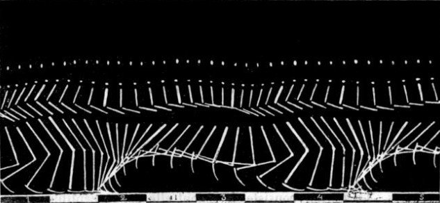 Marey’s Motion Capture with Strips and Lines
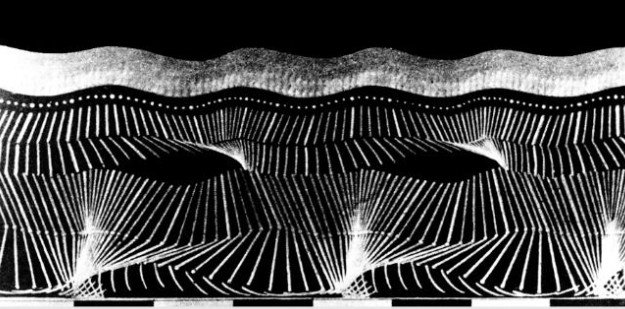 Marey’s Motion Capture with Strips and Lines
In the two diagrams above, Marey turned the motion of the points of change on the body into a diagrammatic expression by using time sequentially. The interval at which he combined the photographs is always equal. Using equal intervals was Marey’s decision, and this shows that he was not concerned with the distance between photographs. Although both show the same movement, the second diagram differs from the first in having both more points of change on the body and less distance between photographs. This results in smoother curves in the resulting graph.
In conclusion, in Marey’s photographs the phases of motion turn into a simultaneous image. This is observed as the traces that motion leaves in space. Here it becomes possible to gain an idea of both the temporal and the spatial characteristics of motion from a single photograph. In the image below, Marey can be seen investigating change in bodies and objects. In the chronophotographs he composed, the temporal unfolding of balances of force is observed.
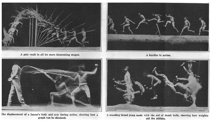 Marey’s Works (Source: Scientific American, 1914)
The chronophotography techniques of Marey and Muybridge show the changes of the time/motion relationship on the body and the object. In both techniques, motion is expressed in the way time is used, sequentially and at equal intervals. However, Muybridge’s technique is more open to topological thinking. Marey’s technique suggests a more Cartesian thinking. In addition, Muybridge created a diagram by arranging the photographs he took in sequence, whereas Marey gathered the photographs he took into a single photographic frame.
kinect motion sensor
Kinect is a motion-encoding sensor that incorporates depth information into the process and transfers spatial movement to the digital environment in real time. With its infrared laser projector and depth camera, it scans the user’s joint points with pattern recognition algorithms. It maps 20 different joint points on the human anatomy in a Cartesian coordinate system (x, y, z).
| regions | |
|---|---|
| head | right knee |
| left shoulder | left foot |
| right shoulder | left ankle |
| left elbow | right ankle |
| left wrist | neck |
| right wrist | right foot |
| right hand | left hip |
| left hand | right hip |
| left knee | hip centre |
| right elbow | chest |
The device converts the spatial and bodily data it detects into real-time point clouds. These point clouds reveal the potential of motion to form volumes and surfaces in three-dimensional space. Within the scope of the thesis, skeleton recognition and surface derivation experiments were carried out with Kinect in order to analyse the software logic of motion capture.
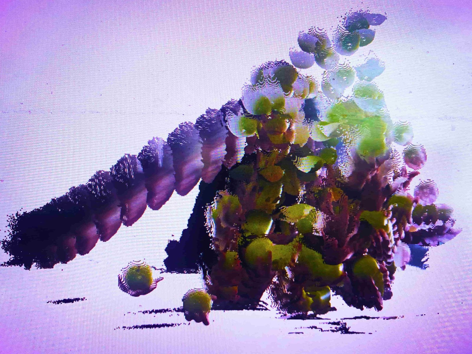 Kinect Point Cloud and Volume Analysis with the Time Parameter
motion capture suit technology
Motion Capture (Mocap) technology converts physical performance directly into numerical data by means of a sensor-equipped garment (suit) worn on the body, without depending on an external camera. The inertial sensors on the suit transmit joint movements to the computer via Wi-Fi, recording Cartesian coordinates with high precision and completeness.
chronophotography experiments
Experiments were carried out on the technique of motion capture through chronophotography. Muybridge and Marey took the photographs they shot with the technology of their time as serial photographs in the direction of the movement. They then expressed the motion by arranging them in sequence or superimposing them. Accordingly, following the chronophotography technique, photographs capturing the movements of the balls were taken for this research. Instead of taking serial photographs as Marey and Muybridge did, a video of the movement was shot and converted into photographs based on the video frames.
To take the photographs, a video shooting area was first prepared. A green screen was chosen to separate the balls from the background in the photographs. In addition, sufficient light sources were provided so that the shadow of the person moving the balls would not fall on the green screen.
A two-second video was shot with the camera. In setting the duration, it was ensured that each ball travelled once from the hand that threw it back to the same hand. The video was shot at 24 fps (24 frames per second), yielding a total of 48 photographs. The video was split into photographs using Adobe Premiere.
The 48 photographs produced for use in the experiments formed two different diagrams using the Muybridge and Marey techniques. In the first diagram below, the photographs are read from left to right to show the temporal fragments of the motion; in the second, the curve formed by the temporal fragments of the motion is observed. These diagrams form the groundwork of the experiments. In these experiments, the curves formed by the motion of the balls depending on the time parameter were investigated. The experiments were divided into two: physical experiments and digital experiments. The experiment parameters read from these diagrams are: trajectory, distance between photographs and number of photographs. The experiments were constructed with references from the concept chapter and through the chronophotography diagrams produced.
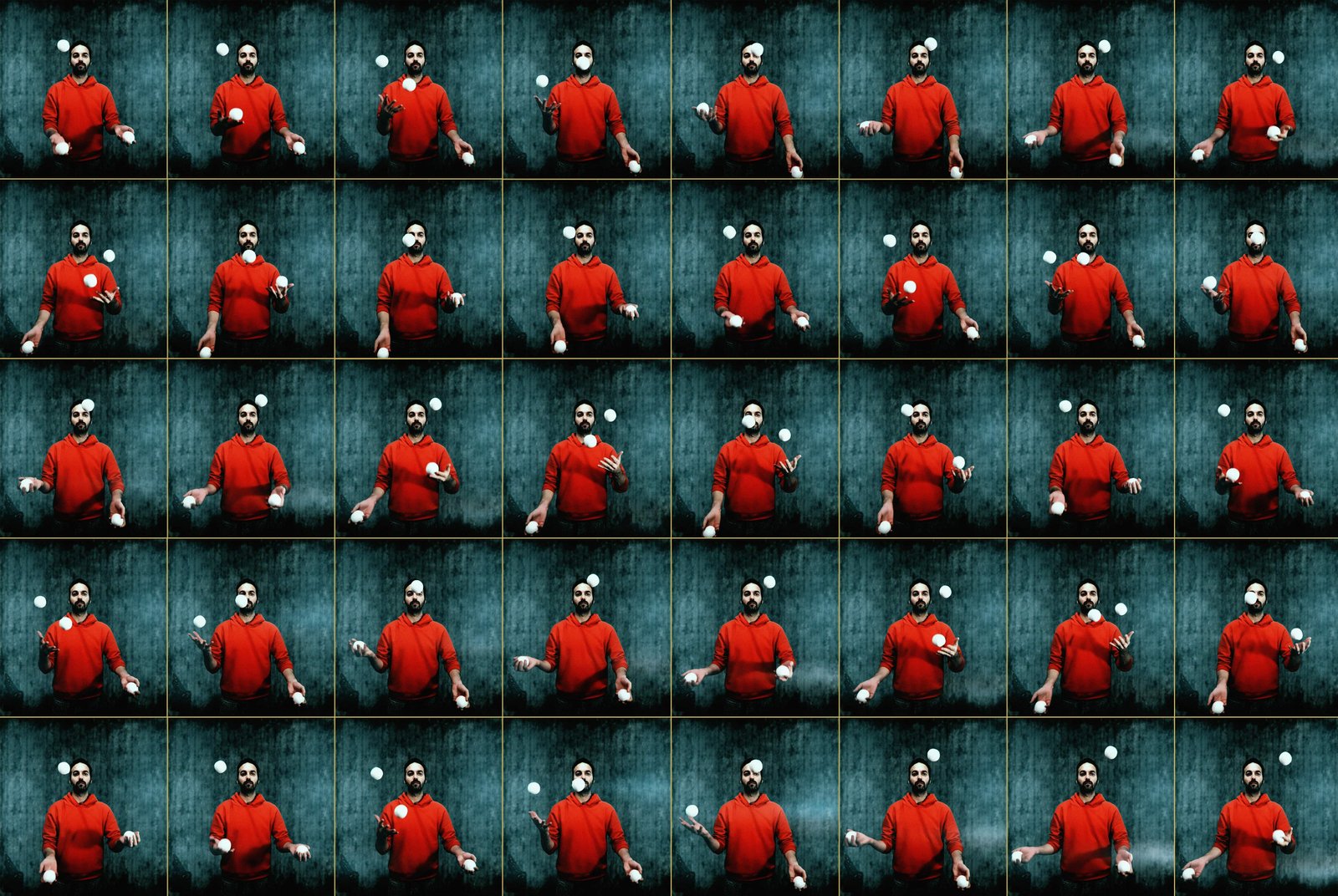 Chronophotography with the Muybridge Technique
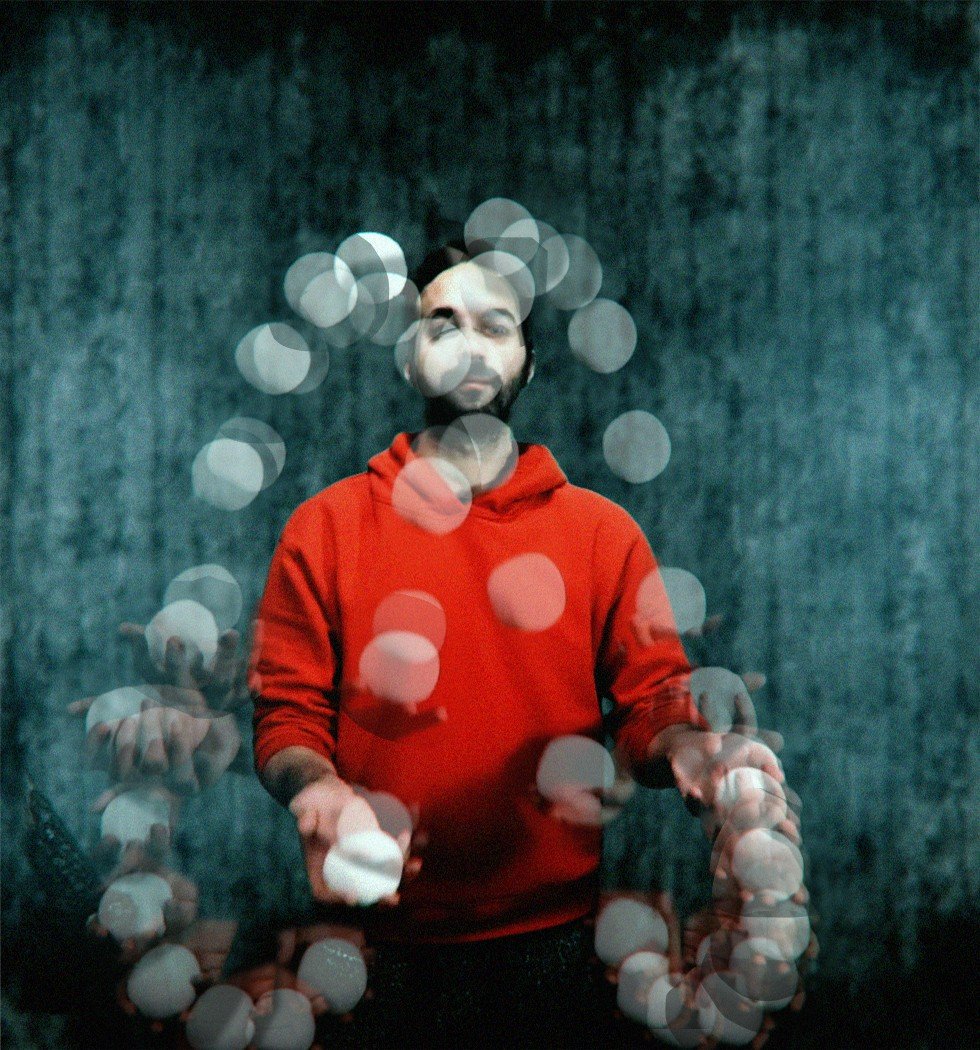 Chronophotography with the Marey Technique
chronophotography physical experiments
These are the initial experiments of the research. They were carried out to examine the time/motion relationship and to observe the curve formed by the trace of the ball. Reading the models produced by the physical experiments made it possible to set up the infrastructure of the digital experiments. Physical models were made of the trajectories (linear, circular, Möbius strip) taken as references from the topological plane section. Since the design parameters would be developed as a result of these experiments, only the basic motion was used.
experiment 1: linear
In the experiment, 18 photographs were placed linearly at 2 cm intervals, with a time difference of 0.11 seconds between them. The aim of this physical model is to observe the trace that the ball's motion forms linearly over time.
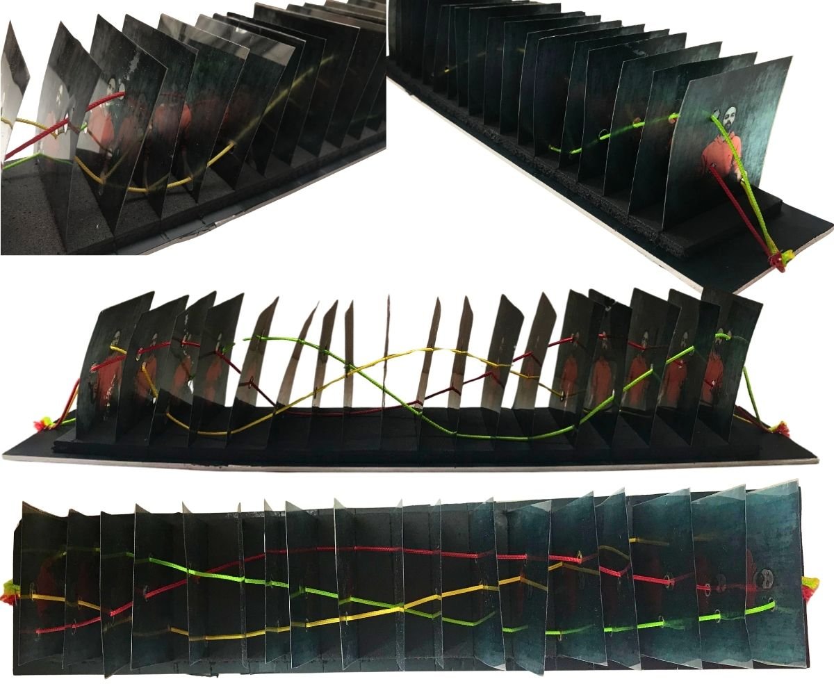 Physical Model of the Basic Motion with a Linear Trajectory
- In the physical model, the strings expressing the ball's motion in the time plane made it possible to perceive the curves that were formed. The relationships between the curves were observed. The distance between the photographs is directly proportional to the curvature of the trace formed by the ball. It was observed that as the interval increases, there are smooth transitions at the control points forming the curve.
- Repetition of the curves was observed in the physical model. Since the photographs were taken from a real-time recording, it was observed that the ball forms a natural curve under the effect of all the forces acting on it. The curve always passed through different points, even if only by millimetric differences. The reason for this difference is that the real-time data carry the force and angle with which the ball was thrown. The fact that the curves formed by the ball's motion follow a linear trajectory made it easier to perceive what kind of curves would form as the motion continued.
- Although the balls pass through the same points in space, the curves of their linearly advancing motions do not intersect one another. In other words, the strings in the physical model do not touch each other. For the curves to intersect, they would have to pass through the same point in space at the same time. If the balls collided with each other at that point, an intersection point would form.
experiment 2: circular
In the experiment, 48 photographs were placed in a circular arrangement. In the physical model, the photographs were placed at an angle, at intervals of 2.75 cm on the long side and 2 cm on the short side, with a time difference of 0.11 seconds between them. The aim of this physical model is to observe the trace that the ball's motion forms circularly over time and to investigate cyclicality.
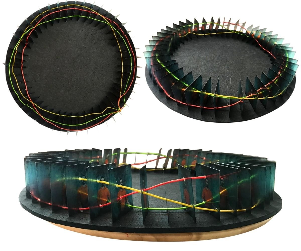 Physical Model of the Basic Motion with a Circular Trajectory
- The strings expressing the motion of the balls formed the curves on the circular trajectory. After the linear model, this laid the groundwork for perceiving the topological plane.
- A circular trajectory means that the start frame and the end frame of the motion are placed at the same point. However, it was observed that the positions of the balls in space were different. This shows that even if the trajectory is circular, there is no cyclicality.
- The distances between the photographs formed an arc. The smaller the arc, the smoother the curves formed at the control points constituting the curve, while a decrease in the interval led to deeper curves.
- Repetition of the curves was observed in the physical model. In this model, since the motion rotates around a centre, the rhythm became more pronounced.
experiment 3: möbius strip
In the experiment, 34 photographs were placed on a Möbius strip. The Möbius strip is a topological condition formed by twisting a linear strip once and joining its ends. Since this experiment was carried out after the digital experiments, it became a model referring to topology. In the physical model, the photographs were placed at equal intervals of 4 cm, with a time difference of 0.28 seconds between them. The aim of this physical model is to observe the trace that the ball's motion forms over time on a topological plane and to investigate the twisting of the curves along the path.
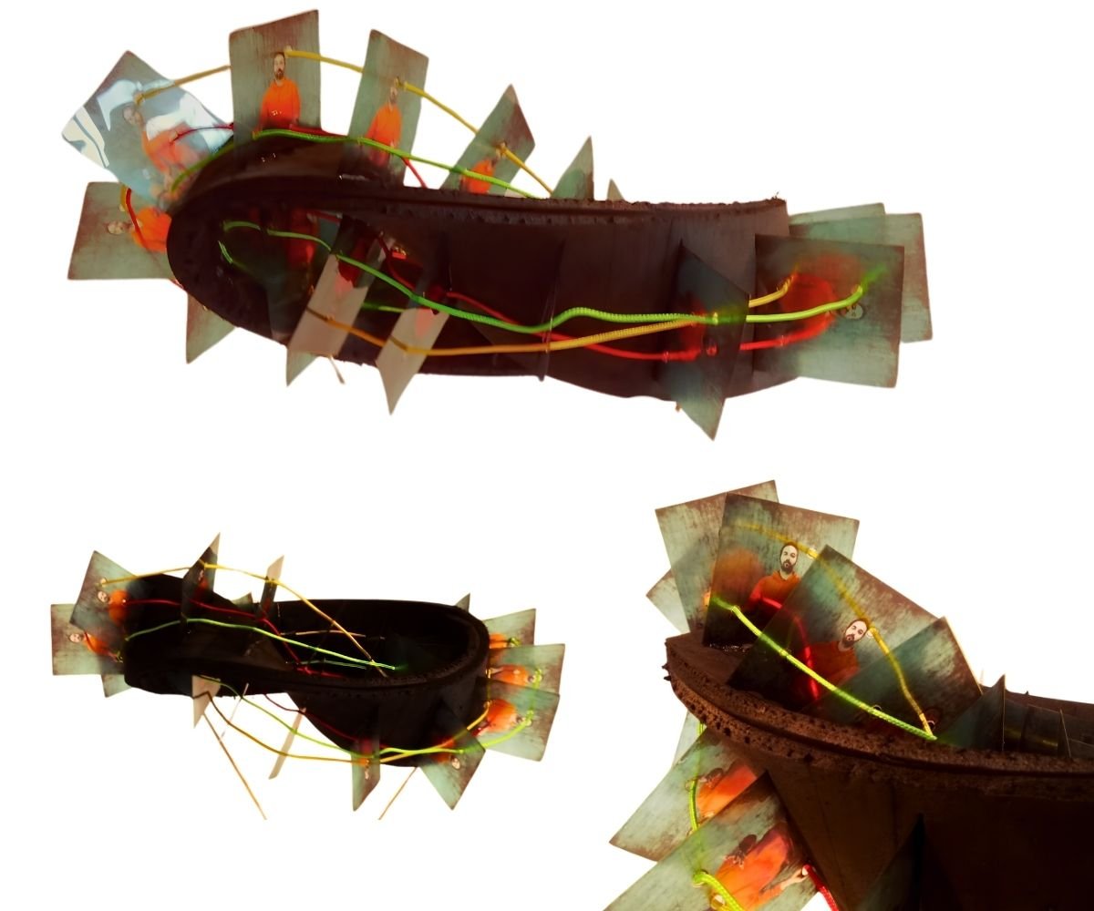 Physical Model of the Basic Motion with a Möbius Strip
- The strings expressing the motion of the balls formed the curves on the Möbius strip. The curves turned along the surface and returned to the point where they started.
- Compared with the first and second experiments, the curves were formed without reference to the ground. At this point, the curves were observed topologically.
- A Möbius strip trajectory means that the start frame and the end frame of the motion are placed at the same point. However, in this model too it was observed that the positions of the balls in space were different.
- Although the distance between the photographs was set equally, it was observed that the distances between the upper points of the photographs had different measurements because the surface was twisted.
- Repetition of the curves was observed in the physical model. In this model, since the motion was rotated on the topological plane, rotation was also observed in the curves.
- The topological effect of the Möbius strip became more comprehensible with the model.
discussion of the physical experiments
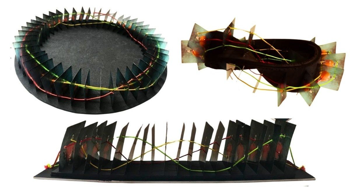 Physical Models - Experiments 1, 2, 3
In these three experiments, the trace of the ball's motion through temporality formed the curves. These curves are clearly observed thanks to the strings. In the experiments, the fact that the distances between photographs differ in all three models shows that the smoothness of the curve changes according to the interval. While deep curves formed in the first experiment, the curves in the second and third experiments are smoother. Since the third experiment was carried out after the digital experiments, the model's relationship with the ground is weaker and it conveyed topological thinking better. In all three experiments the strings do not touch each other; in other words, the curves do not intersect in space. In the first experiment, it is seen that the motion could continue indefinitely on the linear trajectory. In the second and third experiments, although the start and end frames are at the same point, the curves do not join.
experiment 4: marey chronophotography technique
This experiment was built on the diagram created with Marey's chronophotography technique. In this diagram, the curve formed by the ball's motion was observed. On the photograph, the curve passing through the midpoints of the balls was drawn using Adobe Photoshop. In this diagram, which is based on the basic motion, one of the thrown balls started the motion from the right hand and then finished the motion again in the right hand.
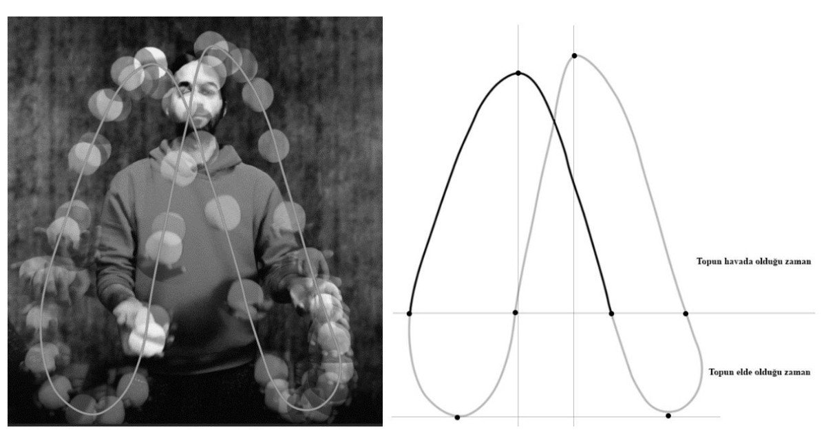 Curve of the Basic Motion
It was observed that the trace of the ball's motion forms a natural curve in the balance of external forces. Since these are real-time motion data, the peak points are not at the same height. The points where the ball leaves the hand are indicated in the diagram. The set-up of the experiment consists of placing the physical expression of this natural curve on the ground at unit intervals. A mould was created by hammering nails into the midpoints of the balls on the diagram glued onto a board.
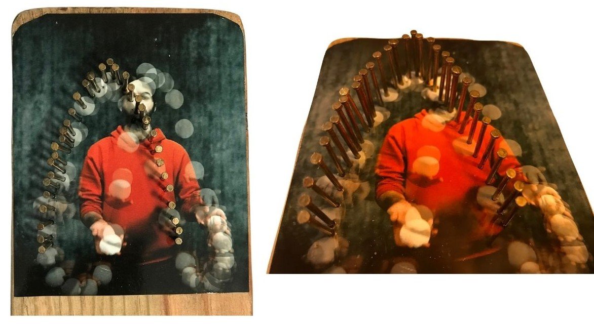 Mould of the Natural Curve
This system is the mould of the observed natural curve. Wires were bent over this mould. The physical model was created by drilling holes in the board at the throwing and catching points of the right and left hands according to unit time. The bent wires were inserted into the holes on the board so as to form three unit time intervals, and thus a graphical model of the ball motions dependent on unit time was created.
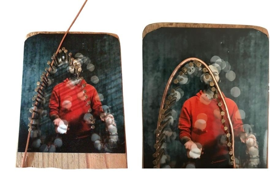 Wires Formed with the Mould of the Curve
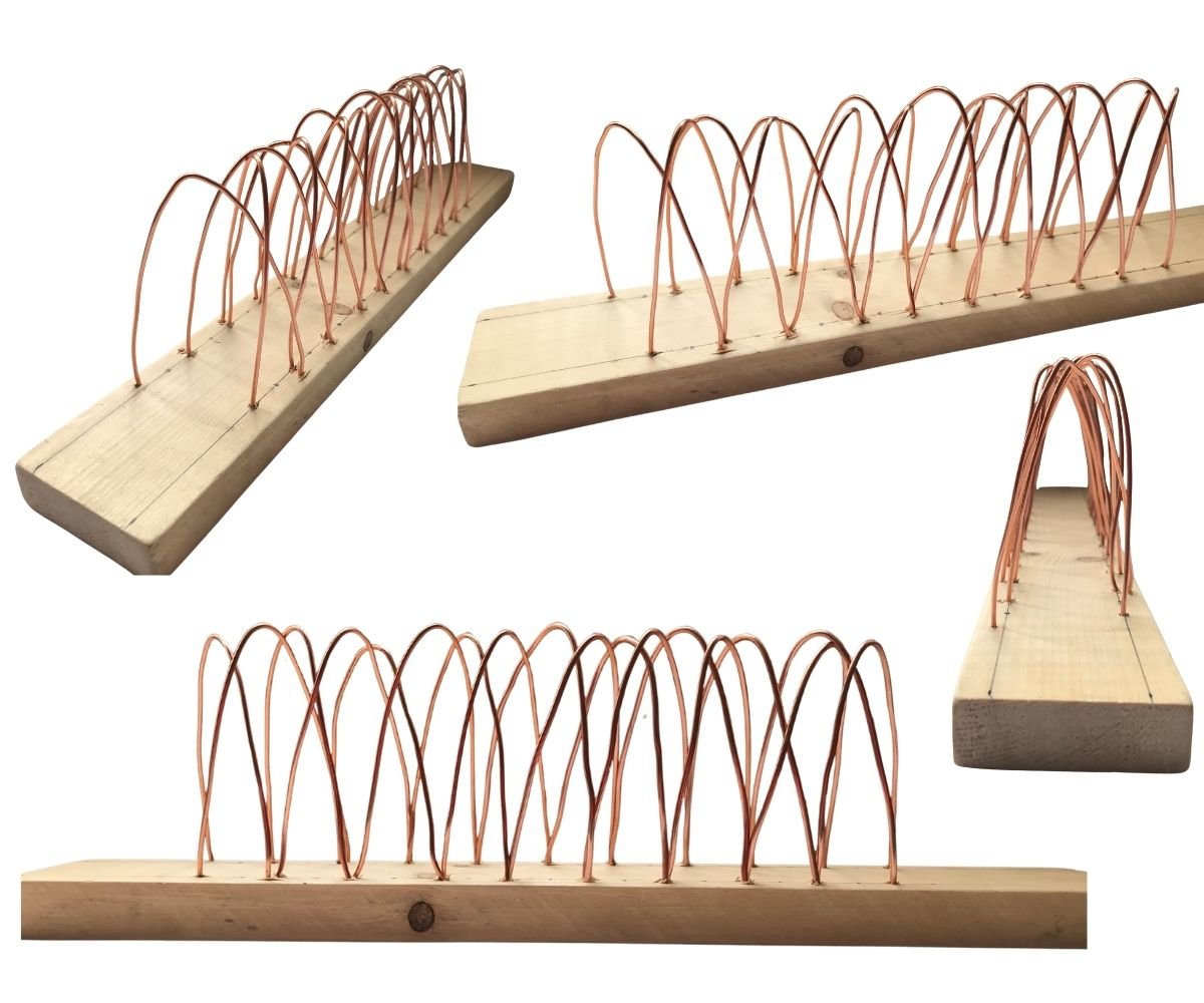 Physical Model - Experiment 4
- The curve emerging in the diagram suggests a parabola equation. This curve is a parabola defined in physics by the equation of projectile motion. The balance of forces on this curve was observed.
- Since it is a parabola formed by real-time motion data, it is not possible to write a general parabola equation. This would require many different parameters to be measured. No additional parabola equation is needed in building the algorithmic software of the research, because the digital software generates the equation of the curve itself.
- The stiffness of the bent wire material creates different curve potentials. The physical model gives the repetition of the basic motion, and this repetition creates a rhythm.
- The natural curves placed in the physical model, by establishing a relationship with the ground, make it possible to propose a structural system.
chronophotography digital experiments
Rhinoceros3D and the Grasshopper plug-in were used in all of the digital experiments. With these six digital experiments, the parameters of the algorithm proposed by the research were investigated and the relationships between them were observed. In Experiments 5-6-7, the physical experiments were repeated digitally and the variables affecting the formation of the curve were made parametric. These three experiments were set up in the same way. First, the photographs are introduced into the Grasshopper plug-in and then converted into point sets. Each point in the point set contains a colour code. With a colour filter, the balls are identified separately and their midpoints are found. Finally, these midpoints form a curve.
In Experiments 8-9-10, curve and surface practices were investigated. These experiments are based on the curves obtained in Experiments 5-6-7. Experiment 8 is a parametric curve study examining the potential between curves. Experiment 9 is a curve study built on the diversity of ball motion. Experiment 10 is an investigation of the curve having a field of attraction and of its relationship with its surroundings.
experiment 5: linear
The 48 photographs of the two-second ball motion used in the physical experiments were introduced into the Grasshopper plug-in and placed linearly. The distances between the photographs were set equal at 1 unit, and this interval was defined as a variable in the algorithm. In addition, the balls in the photographs were coloured so that the separate motions could be perceived.
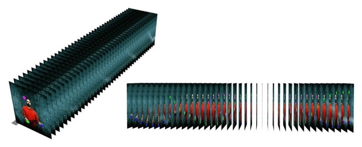 Digital Model of the Basic Motion with a Linear Trajectory
As was done in the physical model, the midpoints of the balls were determined in order to create the curve. To find the midpoints of the balls, the balls need to be separated from the photograph. For this, all the added photographs were first converted into point sets within themselves.
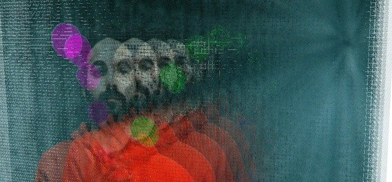 Conversion of the Photographs into Point Sets
Finding the midpoints is the first phase of capturing motion in the digital model with the chronophotography technique. Then a curve passing through the points was created. This curve is the linear digital curve of the ball's motion in the time plane.
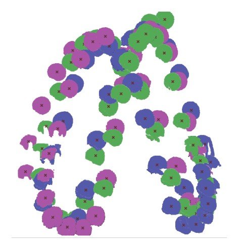 Finding the Midpoints of the Balls
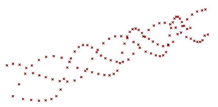 Motion Points of the Balls
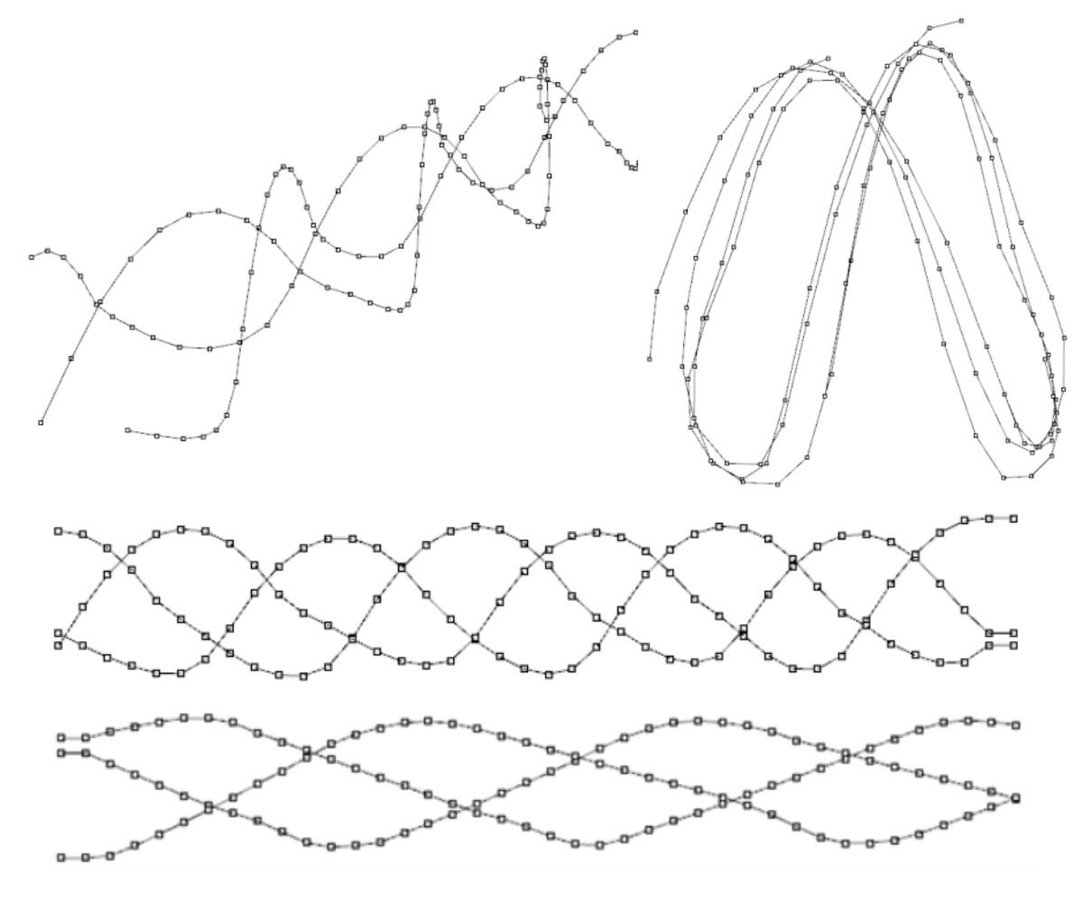 Curves of the Motion in the Digital Model
- Since the model is set up parametrically, new curves can be created quickly by defining photographs of a different ball motion.
- Changing the distance between two photographs affects the smoothness of the curve. Increasing the interval provides smooth transitions at the control points forming the curve, while decreasing the interval provides deeper transitions.
- Definition is important when writing the algorithm. When applying colour filtering to the photographs, a single-coloured and dark background will make it easier to identify the balls.
- Using real-time ball motion data allowed the curves under the effect of forces to form periodically again. However, it was observed that height differences occurred between the repetitions.
- Although the balls pass through the same points in space, the traces of their linearly advancing motions do not intersect one another. This was seen more clearly in the digital model.
- After the curves were created in the digital model, a 3D printer was used to see the physical form of the curves. This made it possible to observe the digital model through a physical model.
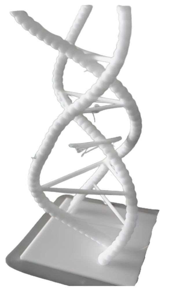 physical model 11
experiment 6: circular
In the Grasshopper definition used for Experiment 5, only the variables of the unit time parameter will change. First, a circle with 48 equally spaced points on it was created, and the photographs were placed at these points.
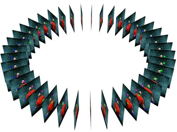 Digital Model of the Basic Motion with a Circular Trajectory
Curves passing through the midpoints of the balls were created. In the digital model, since the start and end of the motion are not the same in the photographs, the curves did not join.
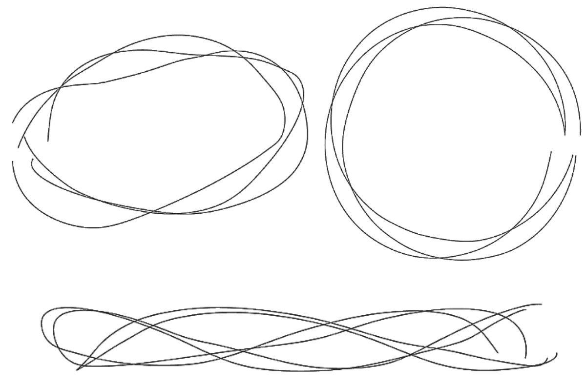 Curves of the Motion in the Digital Model
- Since the model is set up parametrically, new curves can be created quickly by defining photographs of a different ball motion.
- Increasing the distance between two photographs provides sharp transitions at the control points forming the curve, while decreasing the interval provides smoother transitions. At this point, it was observed to be the exact opposite of the linear model. However, if the number of photographs increases in direct proportion as the distance increases, the curves become smoother because the diameter of the circle grows.
- In the digital model the curves did not form a loop, because the midpoints of the balls in the start and end frames of the motion do not provide continuity.
- To the curvilinear nature of the ball's motion in the temporal plane, the curvilinearity of the circular trajectory was added.
- Using real-time ball motion data allowed the curves under the effect of forces to form periodically again. However, it was observed that height differences occurred between the repetitions.
- Although the balls pass through the same points in space, the traces of their circularly advancing motions also do not intersect one another. This was seen more clearly in the digital model.
experiment 7: möbius strip
In the Grasshopper definition used for Experiments 5 and 6, only the variables of the unit time parameter will change. First, 38 equally spaced points are created on the surface of the Möbius strip. Then the photographs were placed at these points along their own axis, perpendicular to the surface. Because of its topological definition, the strip does not form an inner and outer surface; a single surface forms both the inside and the outside.
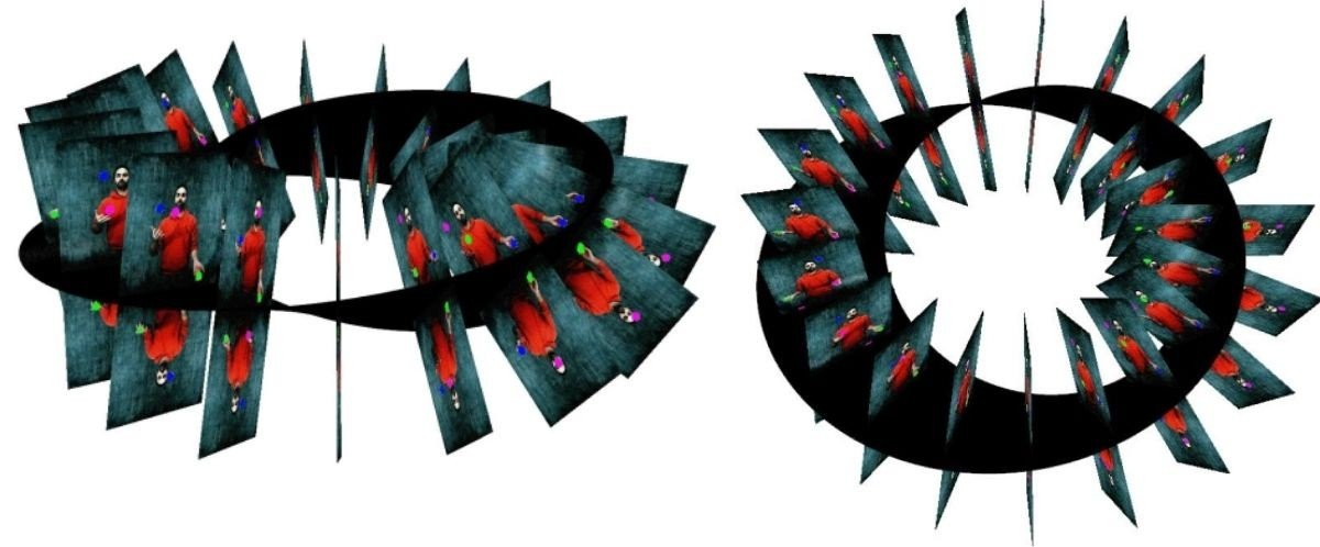 Möbius Strip Arrangement of the Photographs in the Digital Model
As was done in Experiments 5 and 6, the photographs were first converted into point sets, and then, using a colour filter, only the point sets of the balls were identified. The midpoint of each ball's point set was found.
Curves passing through the midpoints were created. In the digital model, since the start and end of the motion are not the same in the photographs, the curves did not join.
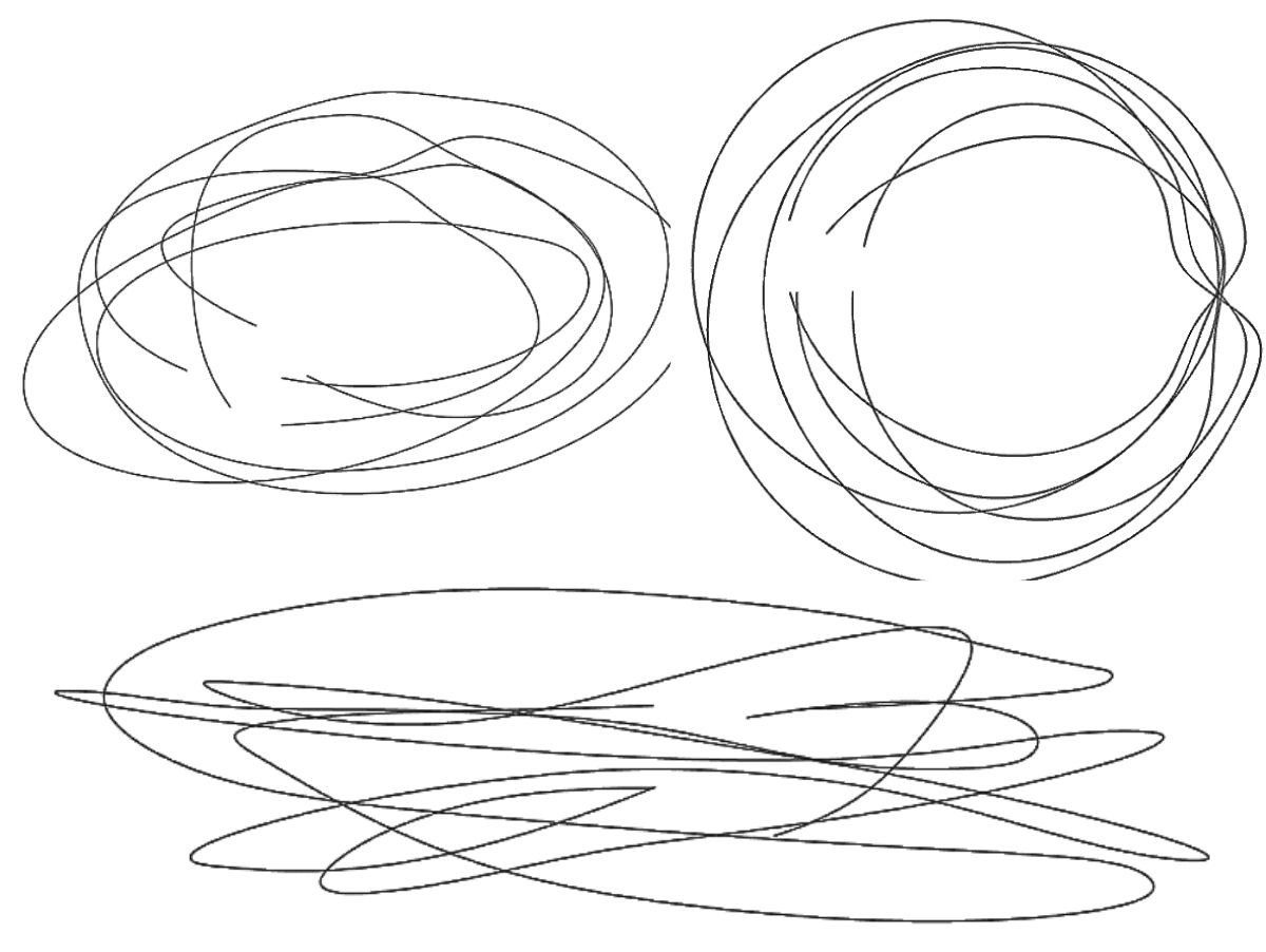 Curves of the Motion in the Digital Model
- Since the model is set up parametrically, new curves can be created quickly by inserting photographs of a different ball motion.
- Changing the distance between two photographs affects the smoothness of the curve in a variable way within itself. Owing to the topological structure of the Möbius strip, as a result of increasing or decreasing the interval, the transitions at the control points behave differently as they progress along the surface.
- Unlike the circular trajectory, variability was observed in the heights of the curves relative to the Möbius strip.
- In the digital model the curves did not form a loop, because the midpoints of the balls in the start and end frames of the motion do not provide continuity.
- To the curvilinear nature of the ball's motion in the temporal plane, the curvilinearity of the circular trajectory and the twisting of the curves were added.
- Using real-time ball motion data allowed the curves under the effect of forces to form periodically again. However, it was observed that height differences and rotations about their own axes occurred between the repetitions.
- No relationship of the resulting curves with the ground was observed.
- It was observed that curvilinearity increased with the use of more photographs than in the physical model.
discussion of the digital experiments (experiments 5-6-7)
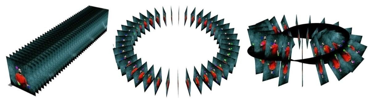 Curves of the Motion in the Digital Model
- In all three experiments, the diversity of the curves formed by different ball motions was achieved parametrically.
- The variability of the distance between photographs determines the smoothness of the curve in the three digital models. In the linear model, as the interval increases, the transition at the control points of the curve becomes smoother; in the circular model, as the interval increases, the transitions deepen; and in the Möbius strip model, as the interval increases, the smoothness of the curve varies. The reason for this is the topological condition of the Möbius strip.
- In Experiment 5, the linear movement of the curve shows that it could proceed indefinitely with the same information. In Experiments 6 and 7, although their geometries are cyclical, the balls in the first photograph are not in the same position as the balls in the last photograph. At this point, cyclicality is not observed in the two models.
- In all three experiments, the ball's motion has its own curvilinearity. In the circular model, in addition to its own curvilinearity, there is a horizontal radial rotation around a centre. In the Möbius strip, together with these two curvilinearities, a vertical radial rotation is observed.
- In all three experiments, using real-time ball motion data allowed the curves under the effect of forces to form periodically again. However, it was observed that height differences occurred between the repetitions.
experiment 8: parametric curve studies
Digital experiments were carried out by setting up parametric relationships with the curves and control points that emerged from the experiments. The curves formed in the time plane of the basic motion and the control points formed on the curves were made parametric depending on variables, and curves were created between the points. The control points are the midpoints of the balls in the photographs. Curve and surface variations open to transformation were produced.
In this variation, the midpoints of the balls in the photograph plane were joined with linear connections. When it establishes a relationship with the ground, both its horizontal and vertical positioning offer a structural system.
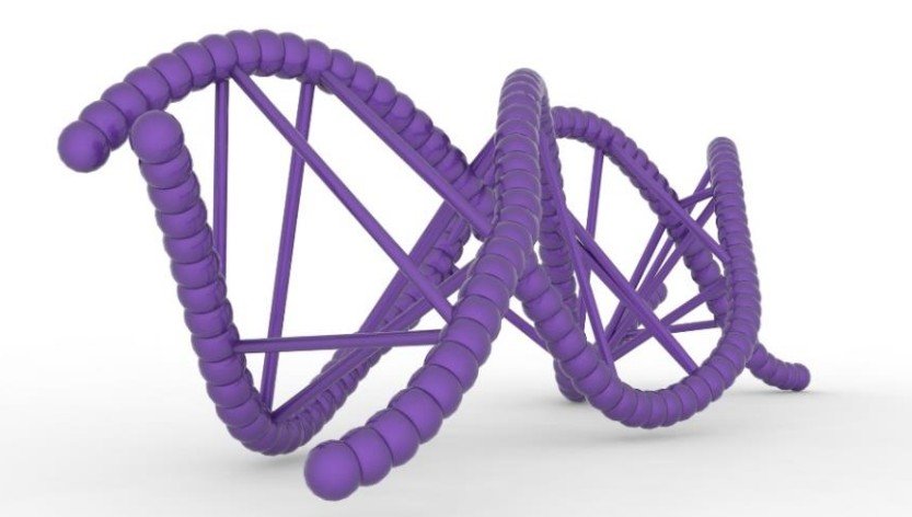 Parametric Curve Study of the Basic Motion
In this variation, the relationship of multiple linear lines from the control points on the curve with the other control points was observed. A mesh-like structure forms between the curves.
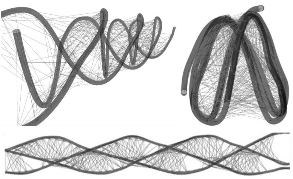 Parametric Curve Study of the Basic Motion
Surfaces were created between pairs of curves. Minimal surfaces were observed.
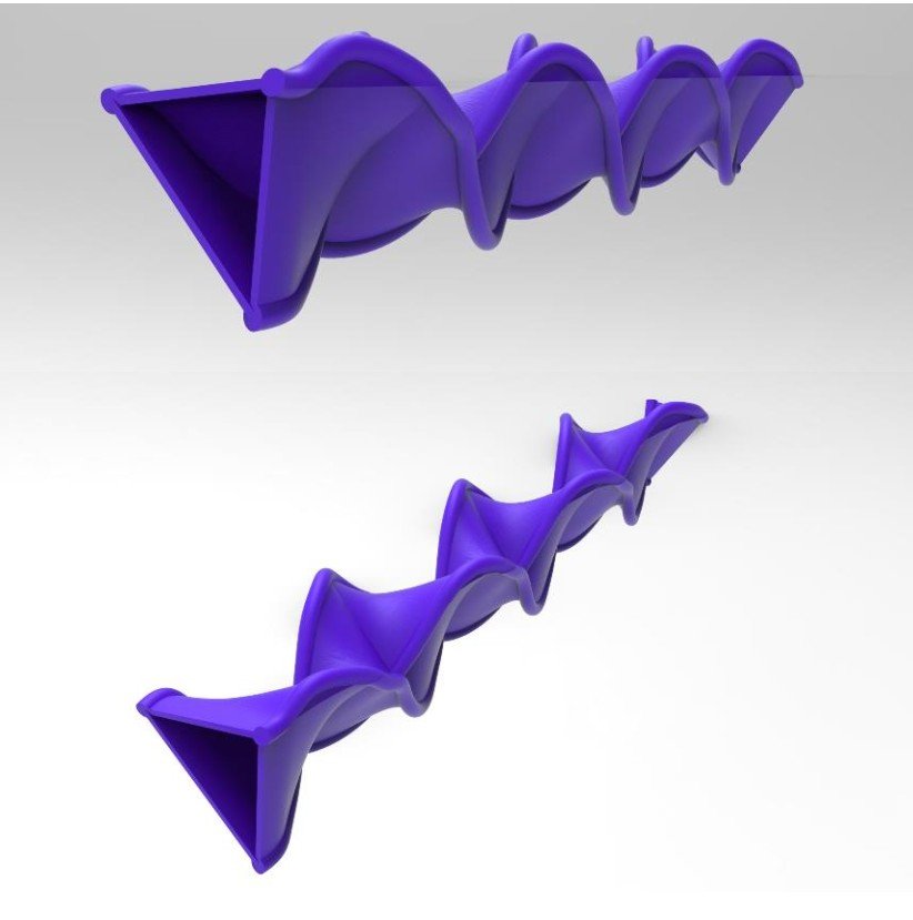 Surface Study of the Basic Motion
experiment 9: choreographic curves
A set of specific movements is called choreography. The relationship of two ball motions that continue without losing continuity in ball motion is observed. In this experiment, the combination formed successively by different ball motions creates a single curve. The curve formed by sequencing the basic motion and the alternative motion one after the other was examined. It will be used in post-thesis research.
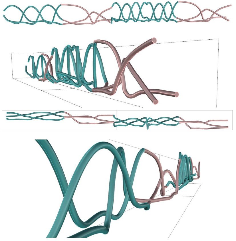 Choreographic Curve Experiment
experiment 10: field of attraction studies
With parametric design, complex ideas that could not be achieved through conventional work have become easy to design with modelling programs. The force of attraction is also a natural force. In this experiment, the interaction of ball motion curves having a field of attraction with their surroundings was observed. The surroundings of the curve consist of linear lines representing flow, and they respond when a field of attraction forms in the curves. The curves formed by the basic motion with the linear trajectory and with the Möbius strip were used.
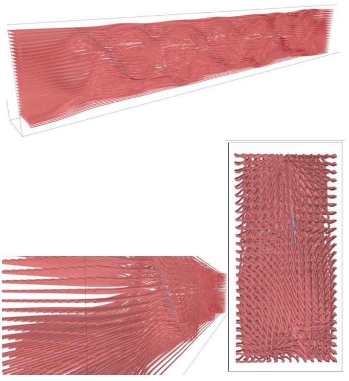 Field of Attraction Study of the Basic Motion with a Linear Trajectory
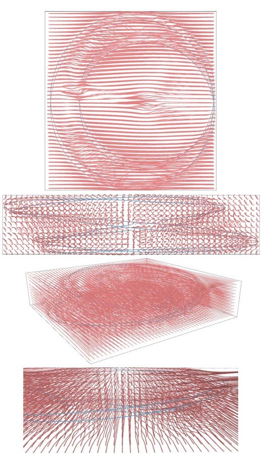 Field of Attraction Study of the Basic Motion with a Möbius Strip
discussion of physical experiments 1-2-3 and digital experiments 5-6-7
- The physical experiments laid the groundwork for the digital experiments and defined parameters for the Grasshopper plug-in.
- In the physical model, to understand the effect of changing the distance between photographs, it is necessary either to make the model again or to imagine it. In the digital model, since this interval is defined as a variable, this effect became much faster to see and easier to compare.
- Since the curves in the digital model are more defined than in the physical models, both the smoothness of the curves and the relationship between the curves were observed more clearly.
- The use of more photographs in the digital model than in the physical model allowed the curve to be formed with more numerical data.
- Repetition is very clearly visible in both the physical and the digital models.
- Converting the curve obtained from the digital model into a physical model with a 3D printer made it possible to understand the digital model better. In other words, although physical models are less defined than the digital model, they are important for discovering potentials when held in the hand.
observation: natural phenomena and dynamic parameters
By experiencing the ball's motion and the curve it forms in space both physically and digitally, algorithms were created together with the digital experiments. These algorithms were used in the observation section to produce variations expressing new curves and information-bearing surfaces. In this section, recordings were made in which the parameters of gravity and wind, among natural phenomena, were analysed; curves were created through the video post-production process.
From this section onwards, the object of observation is called a "sphere" rather than a "ball". The ball is a particular object defined by the way it is used in juggling and in the practice of play; what is observed in this section, however, is not the object itself but the sphere as a geometric body. The sphere is a body that is homogeneous and symmetrical in every direction: gravity acts on its centre of mass, while forces such as wind and air pressure pass through the centre in directions perpendicular to the surface. For this reason, the angle from which the forces come does not create a rotational moment on the body arising from its form. Thus the trace of the recorded motion is freed from deviations arising from the form of the object; only the effect of external forces such as gravity, wind and the throw is read in the curve.
3.1. observation process
To understand the effect of the phenomenon of gravity, the motion and the curve formed by the motion were observed with sets of spheres of different weights, using the basic motion. In this observation, it was assumed that spheres of different weights were thrown with the same force to produce the motion. Although they cannot be thrown with exactly the same force, practice in throwing the sphere with the same force was carried out first, ensuring that the sphere was thrown with nearly the same force. Accordingly, sphere sets of three different weights were specially produced for the experiment. These weights were measured with a precision scale and determined as 30-40 g, 140 g and 240-250 g.
| sphere set | measured weight | number of spheres |
|---|---|---|
| light sphere | 30 - 40 g | 7 pieces |
| medium-weight sphere | 140 g | 7 pieces |
| heavy sphere | 240 - 250 g | 7 pieces |
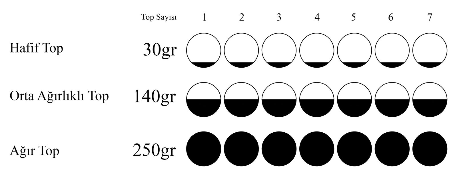 weights of the sphere sets
The effect of the phenomenon of wind was observed in an open area. To observe the effect of wind on the motion of the sphere, recordings were made in both an enclosed and an open area. The enclosed-area recording was made at a venue called Tadah in Antalya. The space was arranged so that no air current formed inside, with the doors and windows closed. The open-area recording was made on the Suadiye shore in Istanbul. A wind strong enough to affect the motion of the sphere was preferred. Wind strength was assessed not as a measured value but by its instantaneous effect on the sphere; the average wind speed during the recording was 20 km/h. Recording real-time data of the wind effect is important, because the variations that will arise from the transformation of the wind effect on the resulting curve unsettle the topological plane.
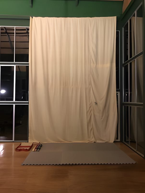
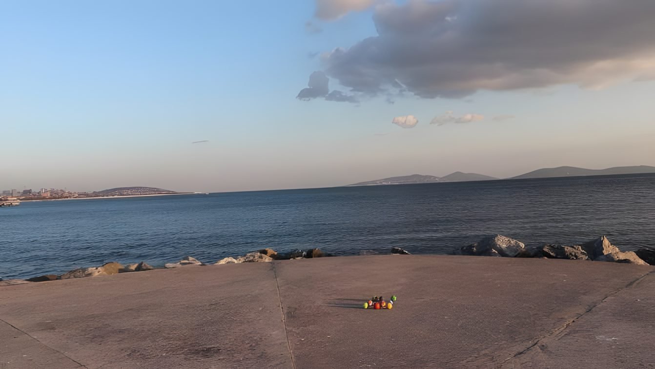
The observation consists of three stages: preparation, video recording and video post-production. In the preparation stage, spheres in different colours were produced so that the spheres could be masked in the video program. Three different colour scales were applied to the sphere sets of three different weights.
 Light Sphere Set
 Medium-Weight Sphere Set
 Heavy Sphere Set
The videos were shot with a Canon 200D at 24 frames per second (24 fps). The motion was defined as the sphere returning from its starting point to the same point. This meant that the motion lasted for different durations in each sphere set. In the video post-production part, a motion capture technique was developed and Adobe Premiere was used. The different colours of the spheres allowed the video program to detect the spheres more easily in the masking stage; in addition, the lighting settings were optimised to separate the spheres from the background in Grasshopper. As the final stage, in order to use the chronophotography technique, the videos were split into frames and made ready for use in Grasshopper.
3.2. observation experiments
As a result of the experiments, the concept of time/motion was observed and algorithms were created. In the algorithm, the midpoints of the sphere were defined and curves passing through these points were created. In the observation section, observation experiments were carried out to define the design parameters and combine them in a single algorithm. The observation experiments were built on defining the effect of gravity and observing the effect of wind.
The design parameters that emerged after the observation experiments defined the heights changing under the effect of gravity by using spheres of different weights, and revealed the effect of wind by observing sphere motion in an open area. With the data obtained from these observations, computable and adaptable design parameters that make the process complex were created; by converting physical data into digital data, the effect of natural forces was made to form the algorithmic process in real time. Rather than proposing a single final curve, the trace of the observed motion proposes the design process that forms the curve.
- motion: Photographs of sphere motion recorded as the basic and alternative motions were used. The data obtained in real time were converted into curves.
- weight effect: The relationship between peak height and mass of the spheres of different weights observed in the enclosed and open areas was set up.
- wind effect: The curve deviations that emerged from observing the light sphere in the open area were examined.
- trajectory: Linear, circular and Möbius strip trajectories provided the spatial differentiation of the curves and the production of variations.
- distance between photographs: By controlling the distance as a variable, the temporal transformation of curve smoothness was examined.
3.2.1. motion
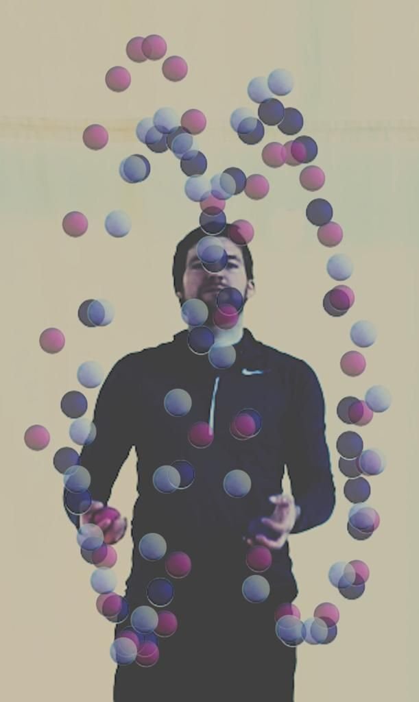
Within the scope of the motion parameter, two different sequences were examined: the basic motion (333) and the alternative motion (423). In the algorithm, this parameter is defined as the serial photographs of the motion. After the video of the desired motion is shot and split into photographs, the algorithm detects the spheres in the photograph and defines their midpoints.
 Basic Motion (Performance: Till Rautert)
 Alternative Motion (Performance: Till Rautert)
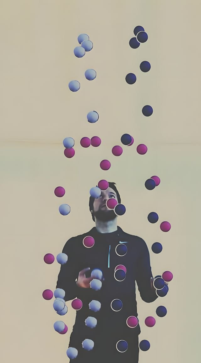
3.2.2. weight effect
Gravity determines the displacement of the sphere in the air. The sphere is thrown from the hand with a pushing force. The effect of this throwing force decreases against the force of gravity as the sphere rises, and at the peak point the vertical velocity drops to zero. Since the effect of gravity continues, the sphere begins to fall. Throughout this process, the balances of internal and external forces are in continuous transformation. This transformation is directly related to the smoothness of the curve and the height of the peak point.
In the experiment, three separate weights were used: the light sphere (30-40g), the medium-weight sphere (140g) and the heavy sphere (240-250g). In the spheres thrown with approximately the same force, it was observed that the peak height decreased as the weight increased. The light sphere reaches the highest level.
 Height Relationship of Spheres of Different Weights
In the curves formed on the linear trajectory, the height differences are clearly legible: green represents the light sphere and blue represents the heavy sphere. As the weight increases, the peak point lowers. Accordingly, the weights 30g, 140g and 250g were transferred to the algorithm as the height parameters h1, h2 and h3 respectively.
3.2.3. wind effect
In order to capture the natural dynamics of the wind effect, physical recordings were made on an open shore instead of a digital simulation. The sphere motion under the effect of wind was recorded in the physical environment and the coordinates at equal time intervals were extracted. The experiment was carried out with the light sphere using the basic motion. Recordings were also made with the medium-weight and heavy spheres; however, since the difference could be clearly observed, these recordings were not split into frames and plotted.
 Basic Motion with the Light Sphere under the Effect of Wind
 Spheres under the Effect of Wind with the Marey Technique
Since the effect of the wind was observed physically, wind strength was assessed not through a measured value but through its instantaneous effect on the sphere. In the same instantaneous wind, the medium-weight sphere was displaced less than the light sphere, and no displacement at all was observed in the heavy sphere. As mass increases, the deflecting effect of the wind weakens. For this reason, wind was accepted as a variable, and it was assessed so that the highest displacement occurs in the light sphere and zero displacement in the heavy sphere.
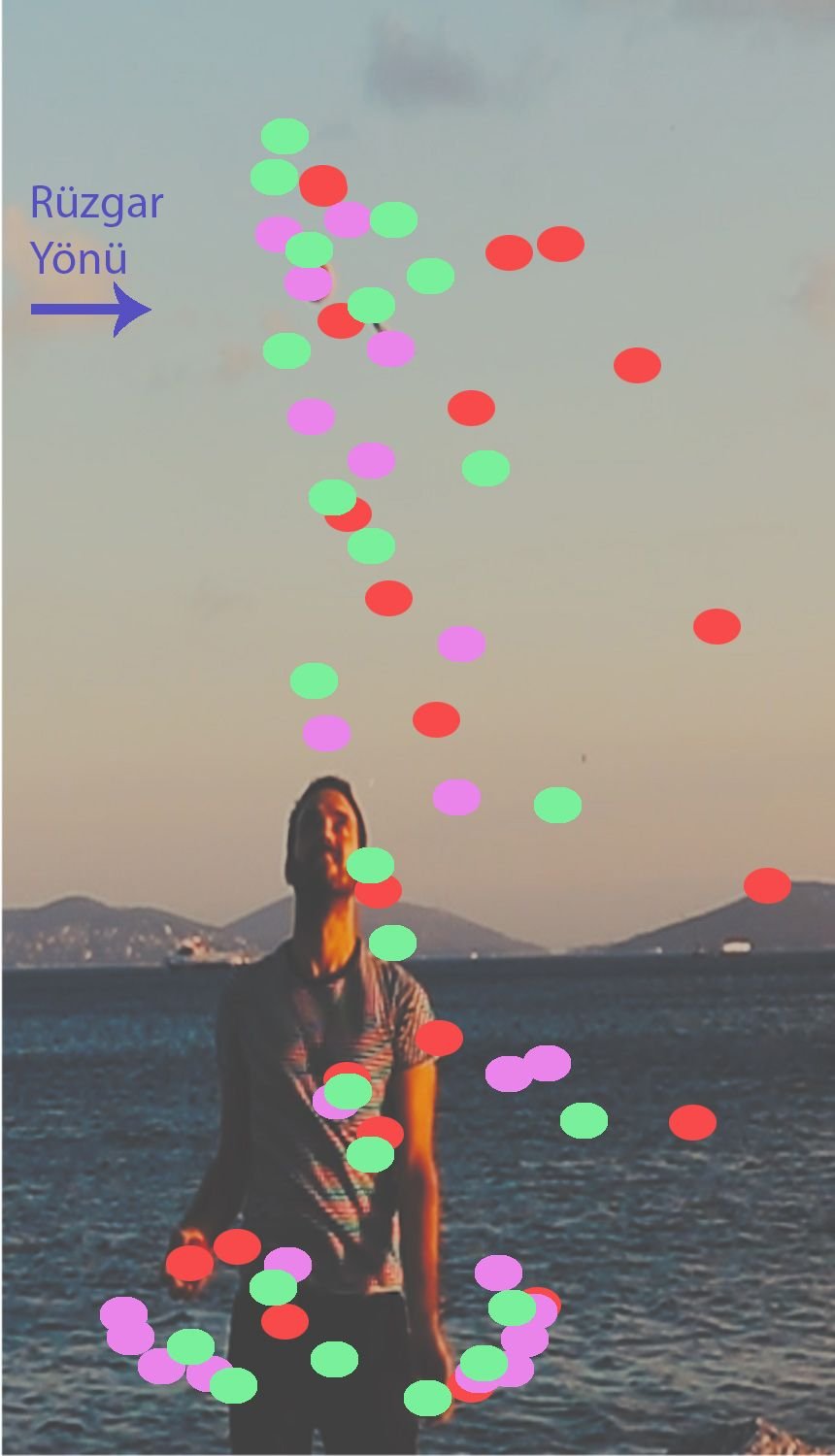

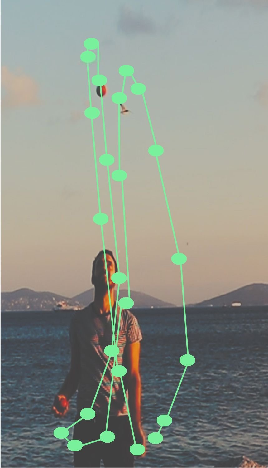
The sphere motion observed in the windless environment of the enclosed area produces a periodic and rhythmic cycle. In the curve under the effect of wind in the open area, however, the deviation becomes pronounced especially at the peak point. This shift in the direction of the wind disrupts the rhythmic repetition; it creates an asymmetric natural curve that makes visible the dynamic interaction of forces.
 Wind-Induced Change of the Curve at the Peak Point
 Curves Formed by the Effect of Wind
 Comparison of the Curves Formed in Enclosed and Open Areas (Purple: Enclosed Area / Yellow: Open Area)
In the comparison in the digital environment, purple curves represent the enclosed area and yellow curves the open area. In the curves under the effect of wind, a sequence of points emerged that do not repeat one another exactly but are computable. These deviations constitute the basic data input of the topological surface set-up.
3.2.4. trajectory
The trajectory parameter was set up as three different trajectories: Linear, Circular and Möbius Strip. Using Muybridge's logic of chronophotography, the experiments carried out with spheres of different weights were repeated in the digital environment. Changing the trajectory diversifies the arrangement set-up in the time plane and allows the curves to be bent topologically.
 Diagram of the Trajectory Parameter
 Basic Motion with the Light Sphere (Performance: Till Rautert)
 Basic Motion Linear Observation Curves
 Basic Motion Circular Observation Curves
 Basic Motion Möbius Strip Observation Curves
 Alternative Motion (Performance: Till Rautert)
 Alternative Motion Linear Observation Curves
 Alternative Motion Circular Observation Curves
 Alternative Motion Möbius Strip Observation Curves
The peak heights produced by the weight differences (light, medium, heavy) on each trajectory were analysed comparatively.
 Basic Motion - Linear Trajectory Comparison
 Basic Motion - Circular Trajectory Comparison
 Basic Motion - Möbius Strip Comparison
 Alternative Motion - Linear Trajectory Comparison
 Alternative Motion - Circular Trajectory Comparison
 Alternative Motion - Möbius Strip Comparison
3.2.5. distance between photographs
Chronophotography is a two-dimensional representation of motion. Muybridge expressed motion by arranging photographs side by side, and Marey by superimposing them in a single frame. In this research, however, photographs taken from a fixed position were placed in the time plane; motion was topologically redefined through the addition of the third dimension and the time axis.
 Trajectories Used in the Research
In the algorithm, the time plane was set up through the distance between photographs and the number of photographs. Both parameters determine the smoothness and total length of the curve. While Muybridge and Marey used equal distances between photographs, in this research, thanks to the topological plane, the distance between photographs can be made variable as desired. This flexibility allows an infinite number of formal variations to be derived instead of a fixed geometry.
model: design process model and surface variations
The term ‘model’ in the section title refers not to a model of a building or object, but to a model of the design process. In the previous experiments, curves were produced from real-time motion data and design parameters were developed by comparing these curves. Up to this stage, the sphere was treated as an object in the photographs; only its midpoint was used to produce time-dependent curve variations of the motion, and no experiment was carried out on the surface producing information. This section is a separate process that investigates how the possibilities determined in the previous sections will produce variations anew through the digital model. The studies here are not a design proposal but basic research showing the process; each surface that emerges is a variation. The main focus is the process algorithm of information-bearing surfaces.
sphere and blob: the information-bearing surface
In this section, the sphere is defined in the digital environment as a body possessing surface information. In the balance of internal and external forces, the sphere has a topological surface every point of which is homogeneously open to the interaction of forces. Greg Lynn defines the sphere in his book Folds, Bodies and Blobs (1998) as follows:
This definition formed the basis for working with the sphere in the digital environment in the research. According to Lynn, the surface of the sphere is transformed by the effect of external forces, as in a water droplet (blob), and is balanced by internal forces. In the experiments in this section, however, internal and external forces are balanced according to the qualitative properties of the material: as the density of the material decreases, the surface softens and the interaction field grows. This increases the sphere's interaction with other spheres, allowing the new surface curves forming between the spheres to have smooth transitions. The interaction field and material density determine the smoothness of the new surface curves. This relationship established between material and interaction field refers to Lynn's definition of the blob; in the research, the sphere is defined as an information-bearing surface.
 Relationship of Blobs with the Interaction Field (Source: Lynn, 1999a: 31)
Brian Massumi (2013) interprets Lynn's definition of the blob in the journal Architectural Design as follows:
In this section, new experiments were carried out with reference to the knowledge of the previous experiments, and the variations this knowledge would produce were investigated. The interaction of the spheres with one another was associated with material qualities, and the parameters discovered in the previous experiments were also included in the process. In the time plane, the distance between spheres is the most important relationship differentiating the interaction.
4.1. distance between spheres
The relationship that gravity establishes with the throwing force reveals the curve of the sphere's motion. From the moment the sphere leaves the hand, the throwing force decreases under the effect of gravity; at the peak point the sphere's velocity becomes zero and the sphere falls under the effect of gravity. When this motion is divided into equal time intervals, it was observed that height differences form between the spheres. This is a natural condition that cannot be controlled.
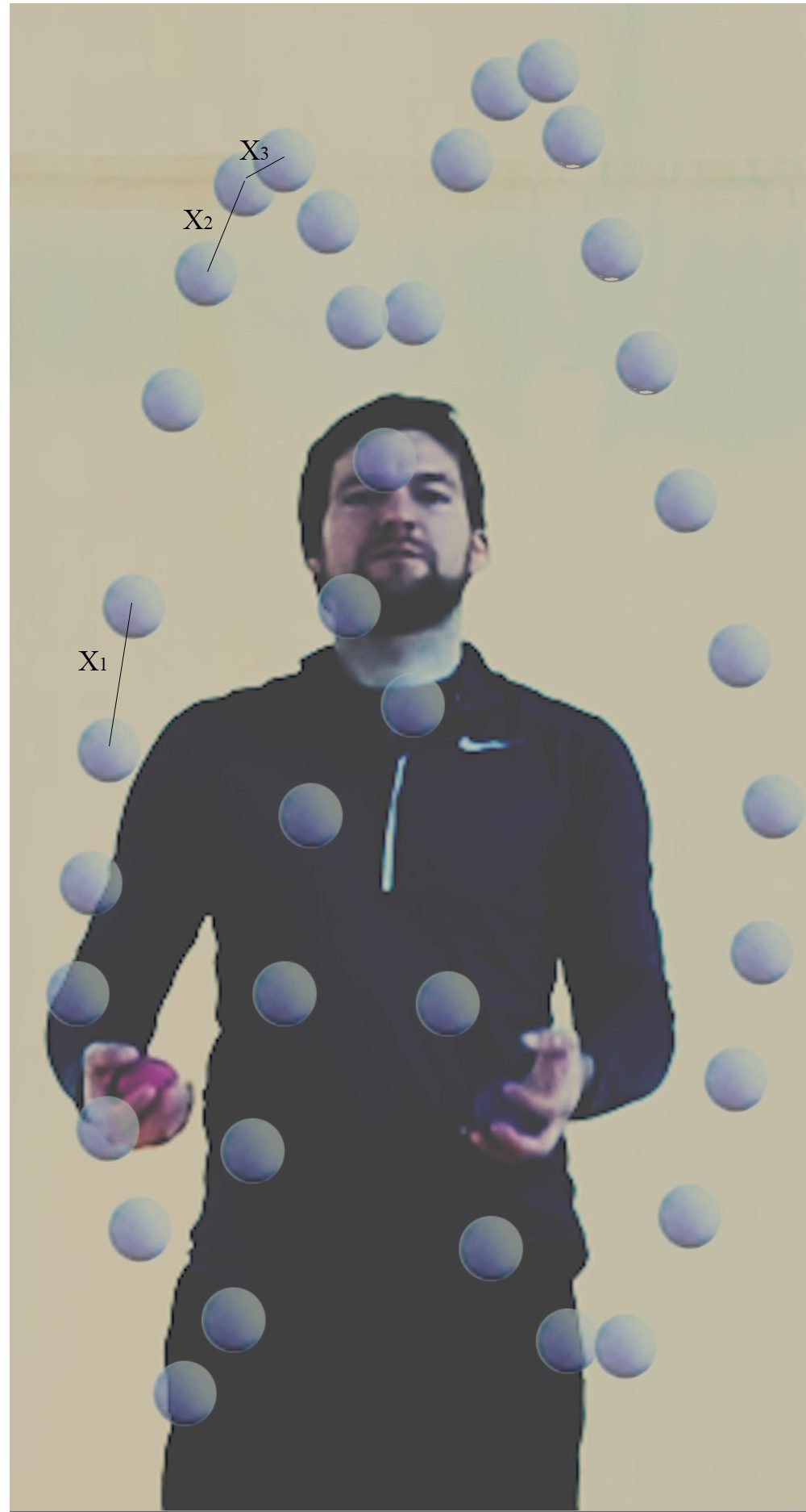 Height Differences between the Spheres
In the diagram above, the distances between spheres are shown from largest to smallest as X1, X2 and X3. As the peak point is approached, the distance between the spheres decreases. This reveals a natural parameter that cannot be controlled but exists; this parameter was used as a variable in the digital environment.
Michael Schumacher defines the relationship between motion and speed in his article The Poetics of Movement in Architecture (2010) as follows:
In the physical environment the spheres are not in a direct relationship with one another; in the digital environment, however, the interaction fields of the spheres become visible. As the effect of gravity increases, the spheres approach one another, and as the distance between them decreases the interaction field grows. When observed in the time plane, this height difference affects the smoothness of the curve forming between the spheres.
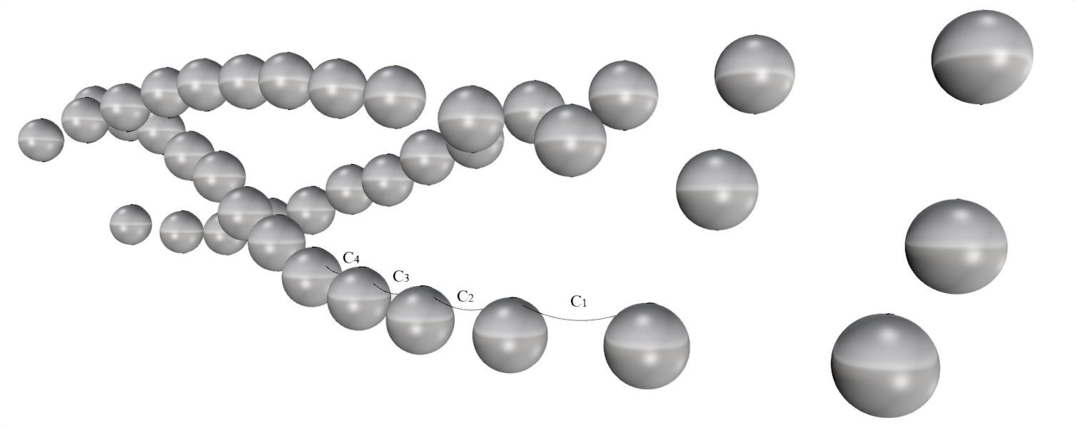 The Smallest Curve
In the diagram above, curves such as C1, C2, C3 and C4 represent the smallest curves. The smallest curve is the topological curve that constitutes the unit of the model in design processes. In this research, however, no single standard smallest curve forms; different small curves form between the spheres and these curves vary according to the parameters.
4.2. surface material
In this section, the surface material parameter was added to the parameters of the previous experiments. The term material refers to the qualitative properties of the material; material density and sphere diameter were used as variables. Material density was defined as a degree of hardness corresponding to the elasticity of the material. The degree of hardness is related to the change in the interaction field of two spheres: as hardness decreases, the interaction field grows and the surface curves soften. No real material data were used in the research.
The spheres used in the previous experiments had hard surfaces; since no work was done with a soft-surfaced sphere, there are no real-time data concerning the surface. In this section, however, the digitally modelled sphere is defined as a body possessing surface information. The material qualities of the sphere transform the balance of internal and external forces; the aim of this parameter is to investigate the topological relationships of the transforming surface.
The change in sphere diameter establishes a relationship with all the other parameters: when the diameter grows, the resulting surface curves are also further transformed by the effect of the variables of height, distance between photographs and material density. To show the difference, spheres of three different diameters were used while keeping the other parameters constant.
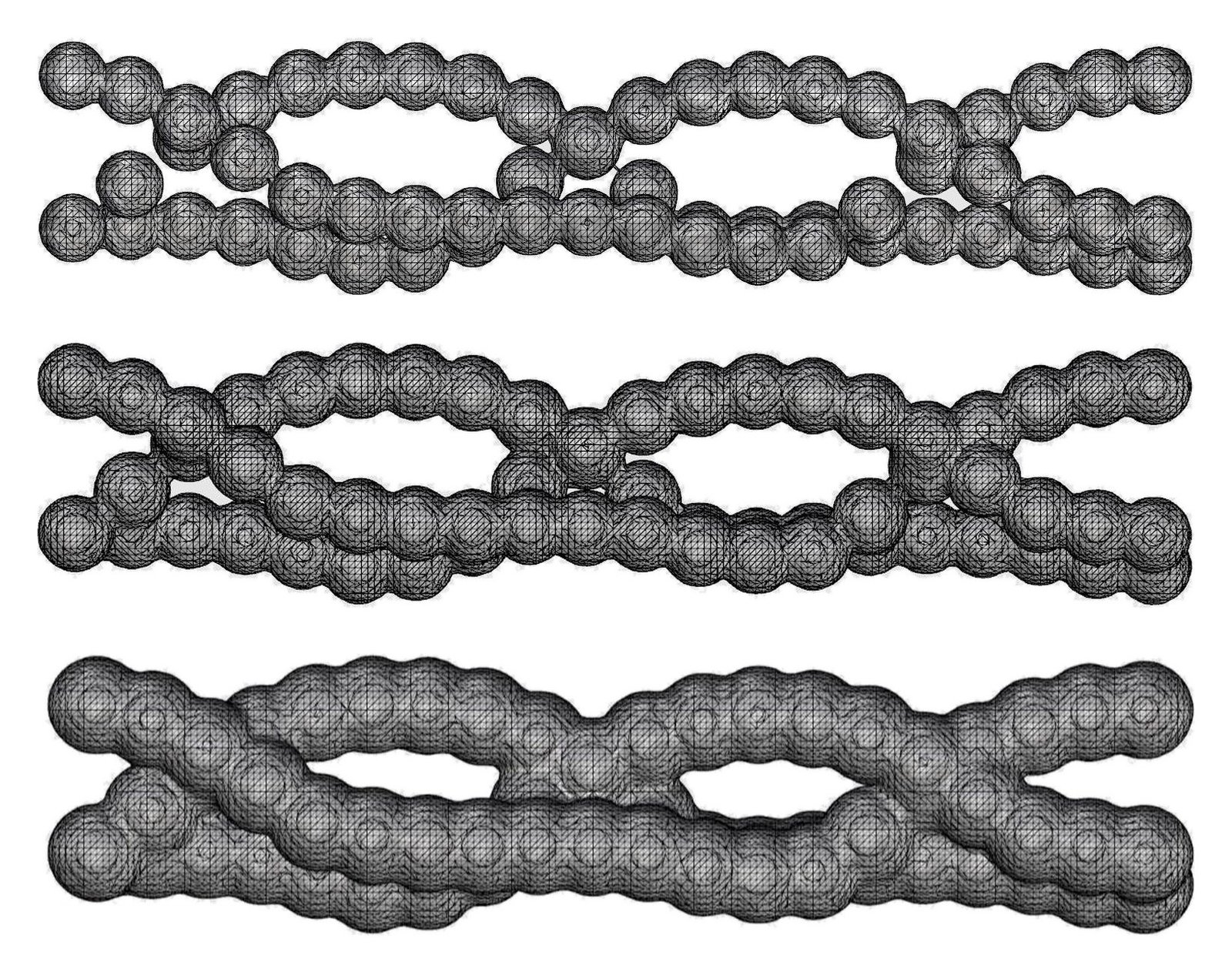 Surface Formation of Spheres of Three Different Diameters
As the sphere diameter grows, the sphere surfaces approach one another even if the distance between the centres remains the same. This enlarges the interaction fields of the spheres and softens the new surface curves that form. In the diagram above, a material of hard density was used; the effect of material density is addressed in the model variations.
4.3. grasshopper definition of the algorithm
The algorithms used in the digital experiments were not changed; an additional algorithm was written for the surface material parameter. First, the sphere midpoints taken from the photographs are placed on the selected trajectory, and spheres of the desired diameter and material density are defined at these points. When the interaction fields are defined, new surfaces begin to form. In the previous experiments the distance between photographs was at equal intervals; in this section the interval was also turned into a variable and unequal intervals were used.
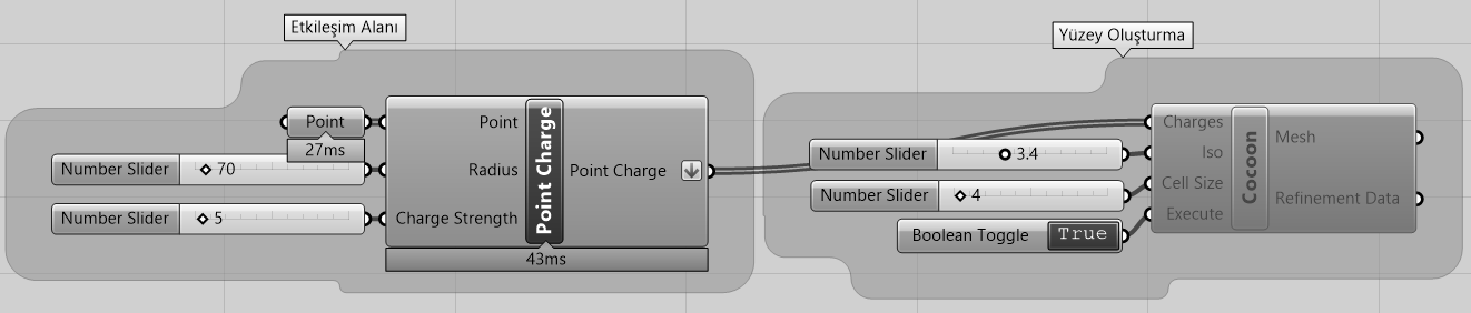 Grasshopper Definition of the Algorithm
In the interaction field algorithm (Point Charge component), the points created on the topological plane are assigned to the Point input, the sphere's diameter to the Radius input, and the attraction strength value to the Charge Strength input. In the surface creation algorithm (Cocoon plug-in), the interaction field information is passed to the Charges input; the coefficients defining the surface are entered into the Iso and Cell Size inputs.
4.4. model variations
By relating all the parameters to one another, ten variations were produced. In each variation 39 photographs were used; the variables are summarised in the table below. The values h1, h2 and h3 in the weight effect column refer to the peak heights measured in the weight effect experiments.
| variation | motion | weight effect | wind effect | trajectory | distance between photographs (unit) | sphere diameter (unit) | material density |
|---|---|---|---|---|---|---|---|
| 1 | basic | h1 | open area | linear | 35 | 55 | hard |
| 2 | basic | h1 | open area | circular | 25 | 20 | hard |
| 3 | basic | h1 | open area | linear | 35 | 55 | soft |
| 4 | basic | h1 | open area | circular | 25 | 20 | soft |
| 5 | basic | h1 | open area | linear | 35–15–25 (variable) | 20 | soft |
| 6 | basic | h2 | enclosed area | möbius strip | 25 | 20 | soft |
| 7 | alternative | h3 | enclosed area | linear | 35 | 20 | soft |
| 8 | basic | h3 | enclosed area | linear | increasing from 35 | 50 | soft |
| 9 | alternative | h2 | enclosed area | linear | 25–55 increasing | 20 | between hard and soft |
| 10 | alternative | h3 | enclosed area | linear | 35 | 20 | soft |
You can rotate the model by dragging. To zoom with the mouse, first click once on the box; the button in the corner enlarges the box to full screen. On a touch screen, enlarge the box to turn the model.
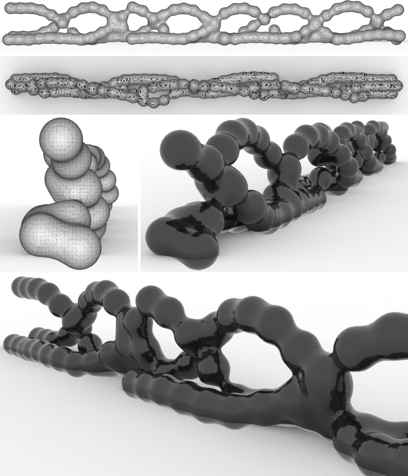 Variation 1
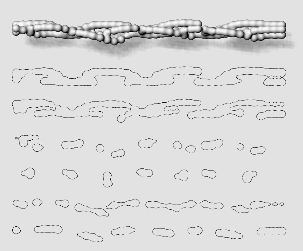 Variation 1 Sections
 Variation 2
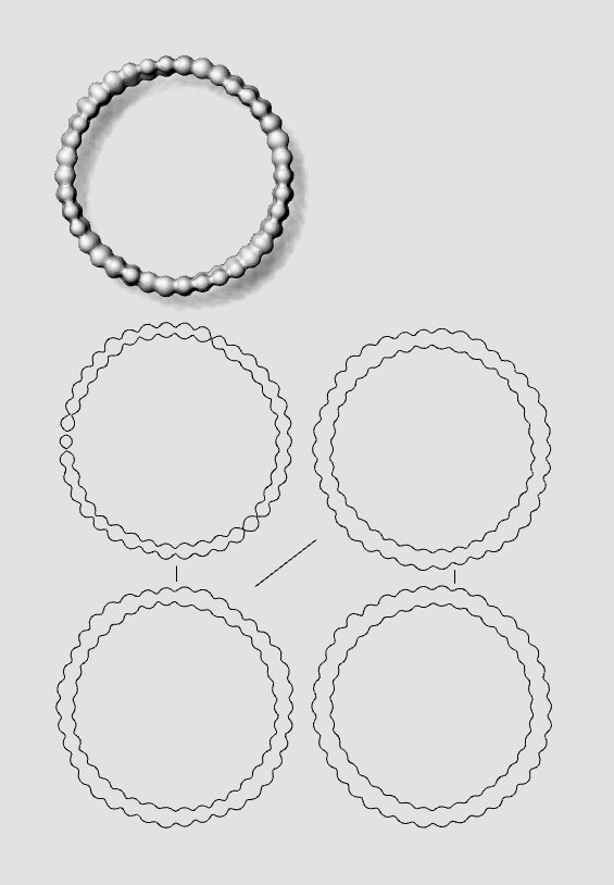 Variation 2 Sections
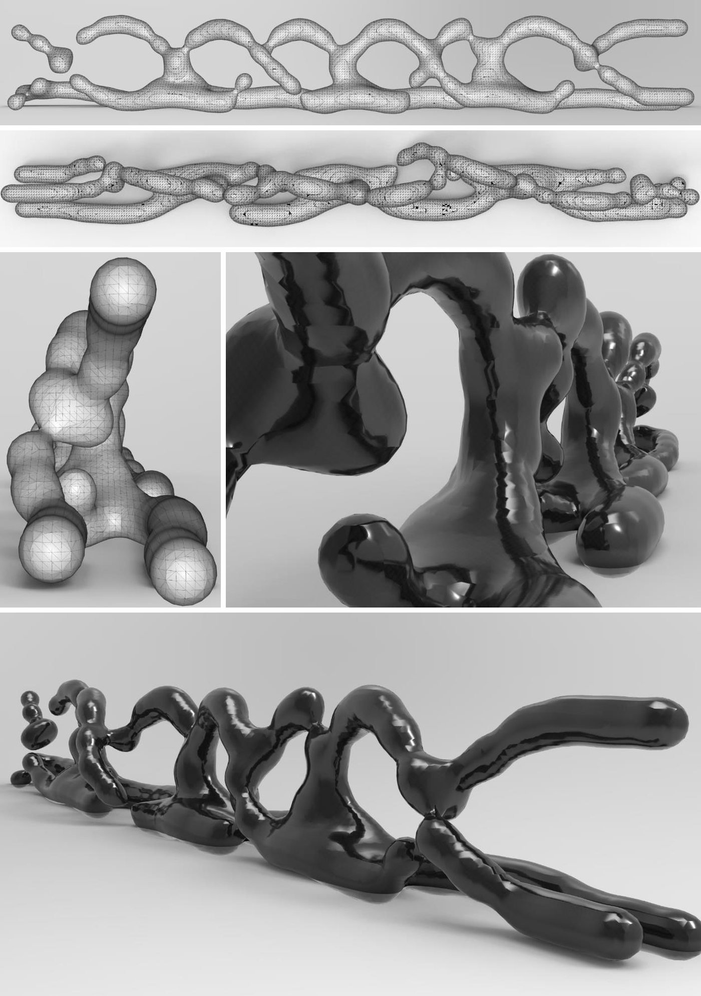 Variation 3
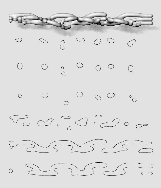 Variation 3 Sections
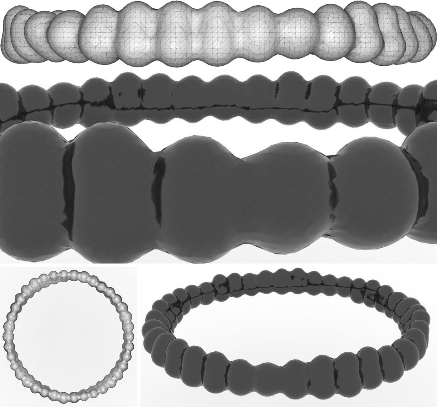 Variation 4
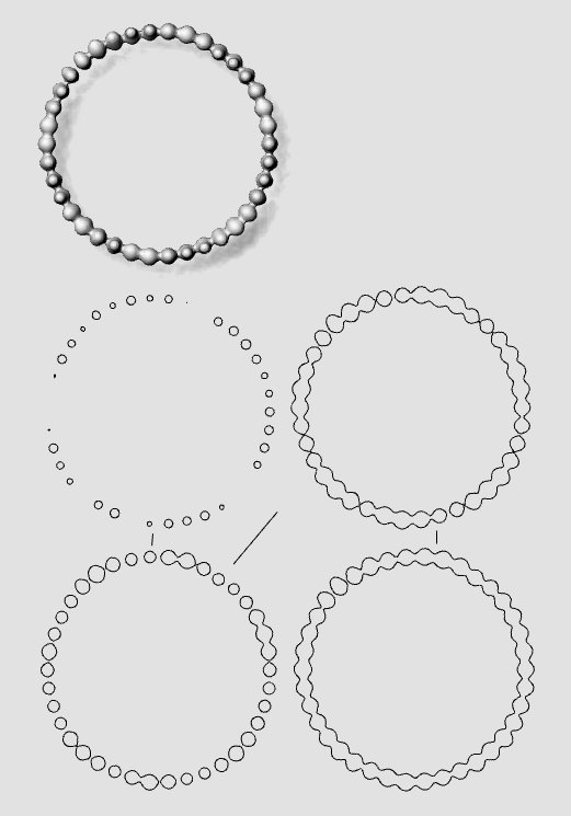 Variation 4 Sections
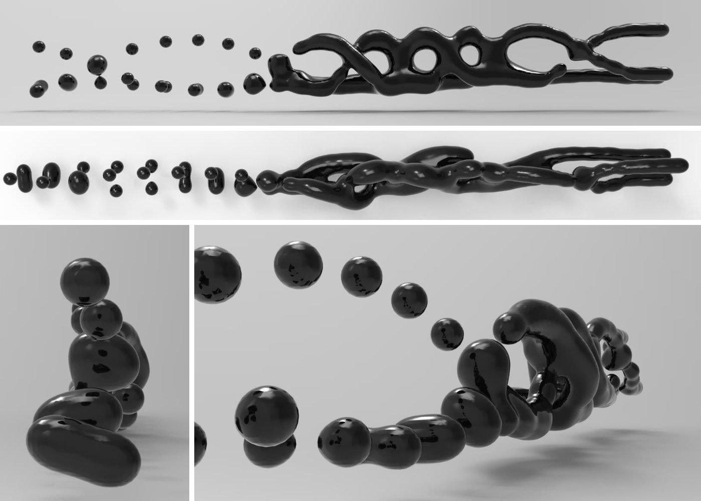 Variation 5
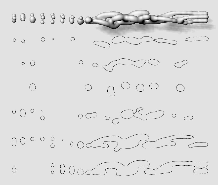 Variation 5 Sections
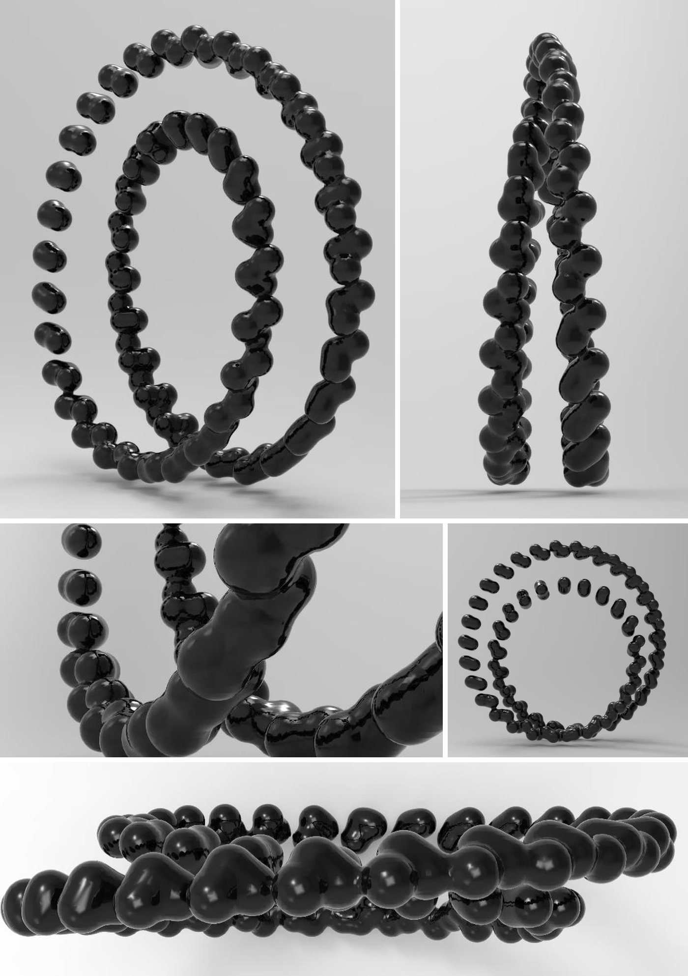 Variation 6
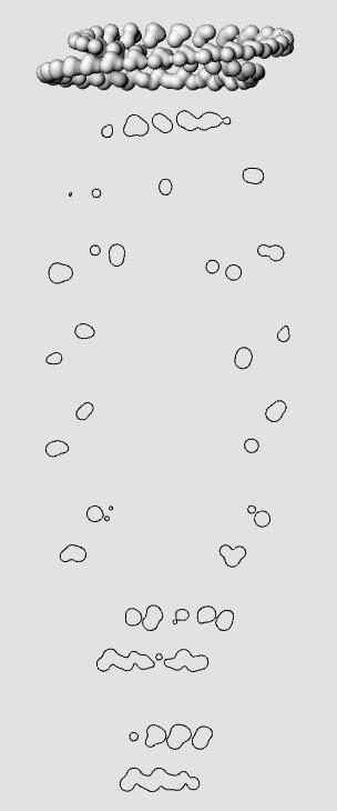 Variation 6 Sections
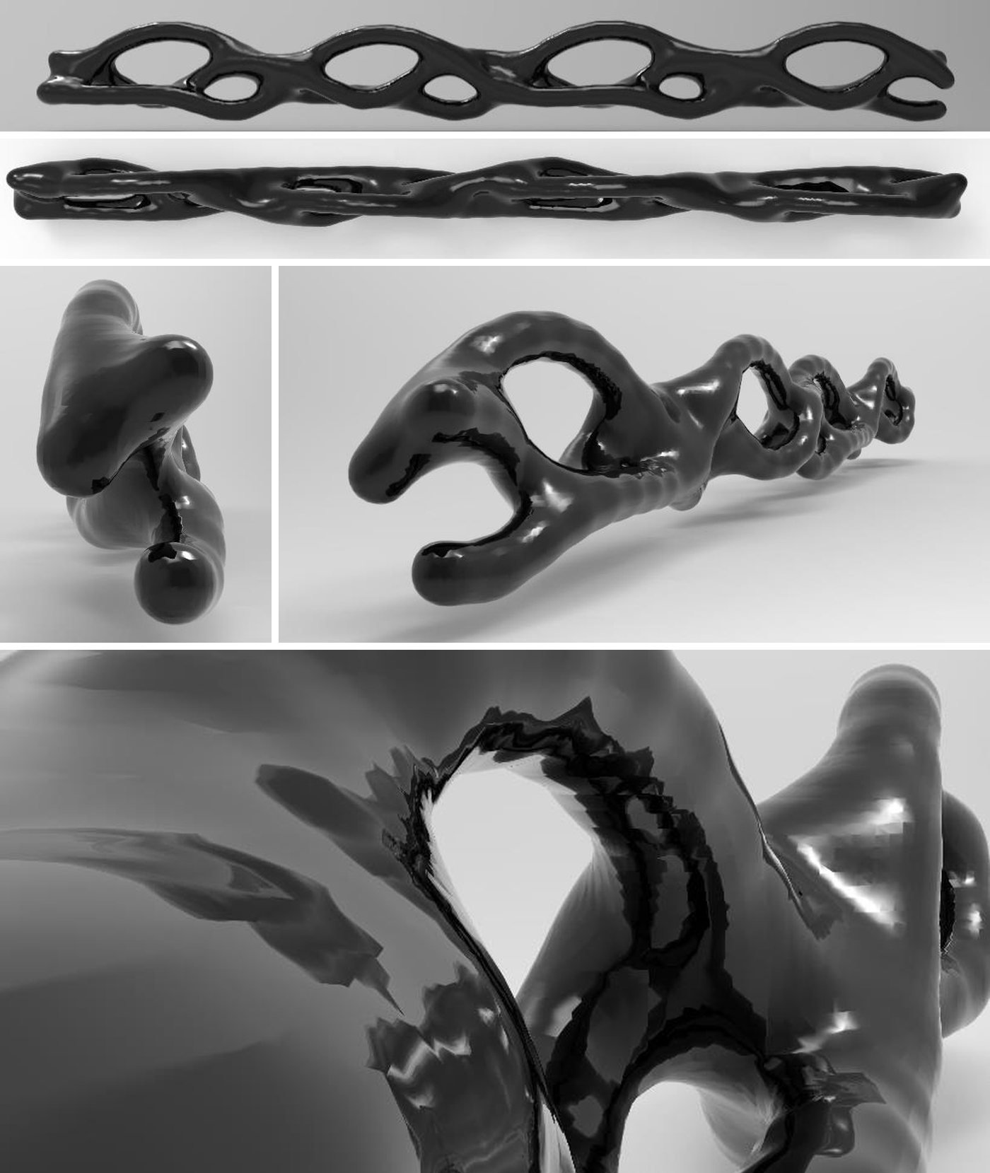 Variation 7
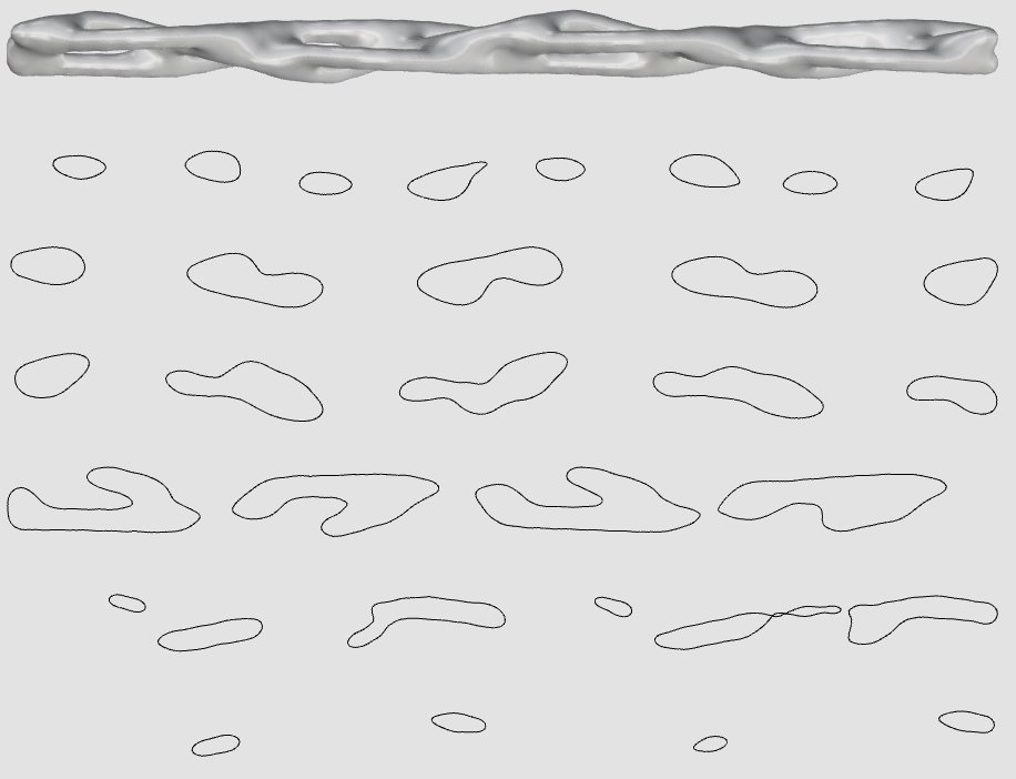 Variation 7 Sections
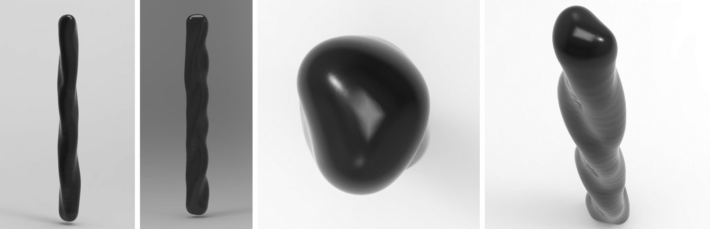 Variation 8
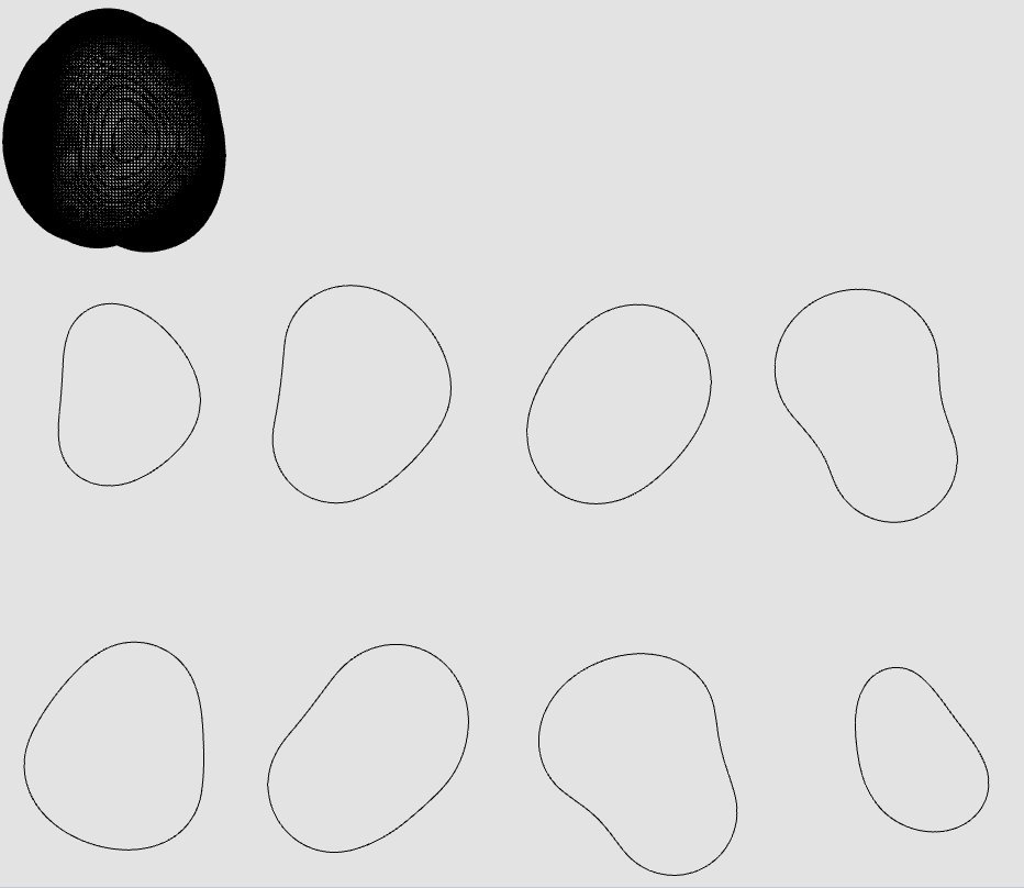 Variation 8 Sections
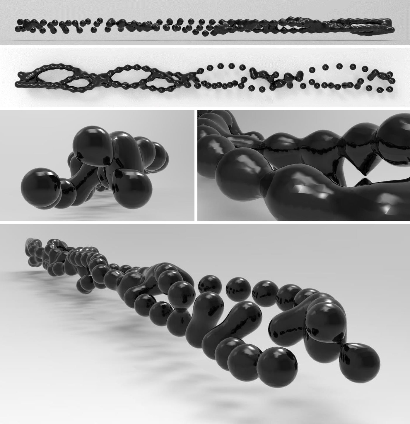 Variation 9
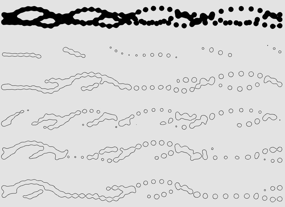 Variation 9 Sections
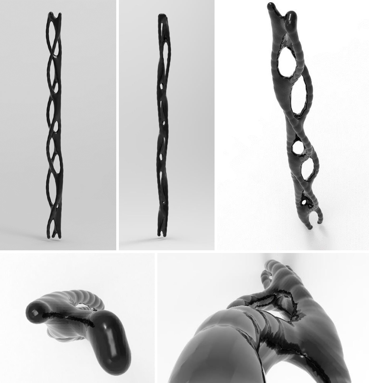 Variation 10
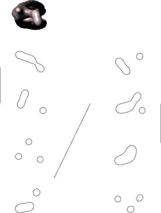 Variation 10 Sections
4.5. comparisons and outcomes
In the variations with hard material density (1 and 2), the section curves are deeper.
In Variation 9, material density was given a value between the hard and soft values; in the sections a transition from a deep curve to a soft curve is observed. This shows that decreasing material density creates soft surface curves.
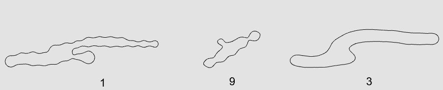 Effect of Material Density
In Variation 8, the sphere diameter is larger than in the other variations. The increase in diameter shortened both the distance between the photographs and the distance between the spheres themselves, and enlarged the interaction field; as the number of interacting spheres increases, the interaction fields expand.
In Variations 1 and 10, different motions and different height values were used. Height is the value of the weight effect parameter: in these two variations the light and heavy sphere curves from the observation experiments were used, and the height of the heavy sphere is less than the height of the light sphere. The difference in the material density, weight effect and motion parameters clearly shows the difference between the two surfaces; Variation 10 has softer curves. The differences in the interaction fields of different motions also provide the diversity of the resulting surfaces.
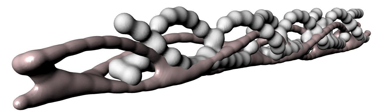 Variation 1 and Variation 10
The distance between photographs is an important finding in terms of variation diversity. In this section, the algorithm defined the distance as a variable instead of setting it up at equal intervals. In Variation 9 the distance gradually increases; as the interval increases, the interaction between spheres decreases.
 Variation 9 Section Diagram
From point a to point g, the interval increases regularly. From point b onwards, the smoothness of the curve begins to change. At points c and e, the proximity of the curves to one another, and at points d and f, the decrease in the distance between the spheres themselves, enlarged the interaction fields.
Since the research was carried out on the topological plane, whether the variation models stand vertically or horizontally does not affect the resulting surfaces; this is only for representation. The perception of ground and the shading in the images are for the perception of depth and do not propose a Cartesian plane.
In the sections of Variation 6, the curves reflect the topological twist of the Möbius strip; this twist is also observed in the digital model.
Repetition is observed in all variations; however, no repetition resembles another.
In Variations 2, 4 and 6, the act of topological rotation created angled intervals; in the sections of these variations, it is observed that curve smoothness differs.
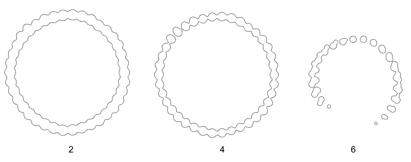 Angled Interval Condition
4.6. variation diagram
The ten variations are shown together with their parameters in the diagram below.
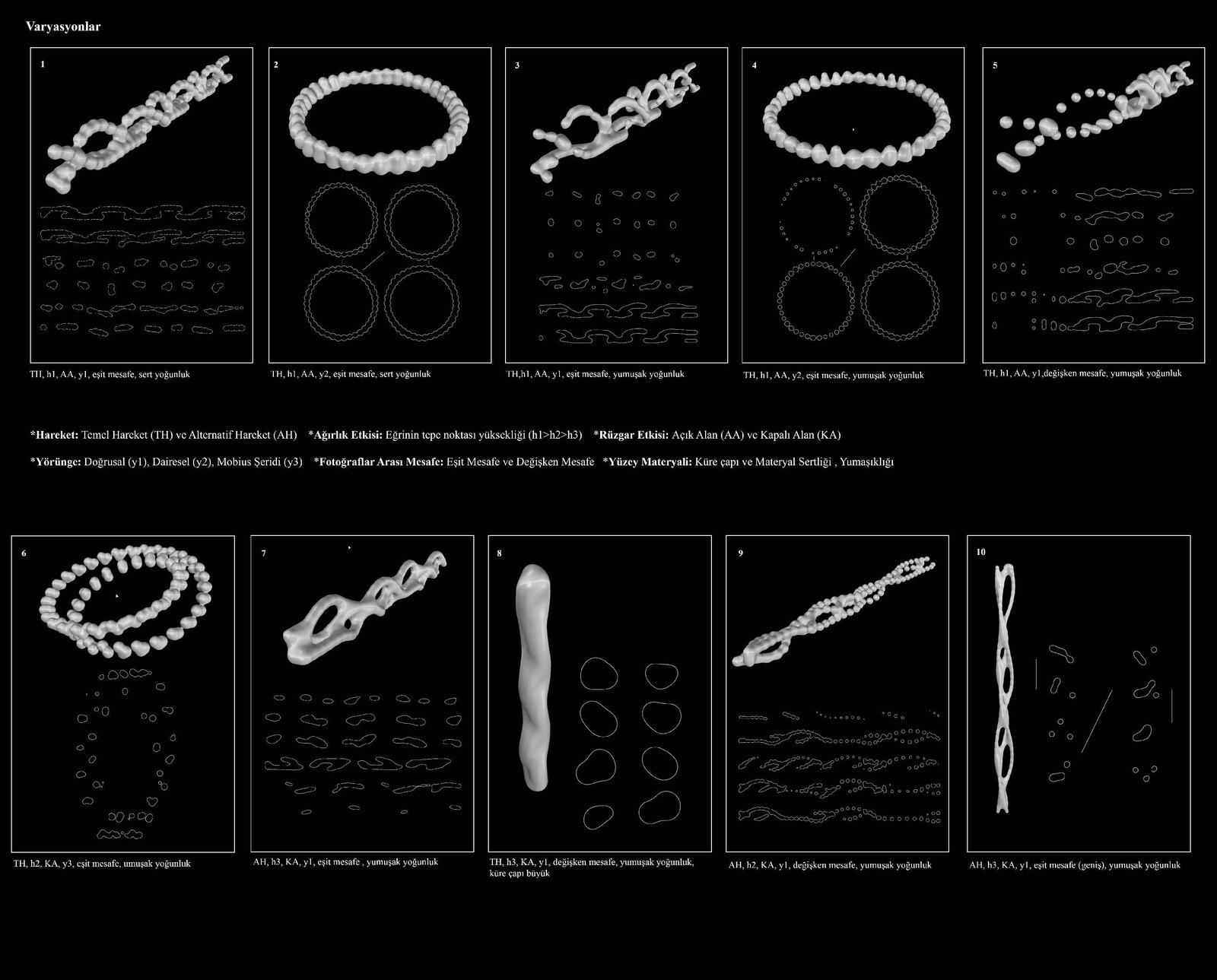 Variation Diagram
conclusion
The research is based on an approach that synthesises conventional and innovative design practices and uses physical and digital expressions together. Through the relationship between concept and production practices, ‘time/motion’ is the basic concept of the research. In this context, process models depending on the potentials of a sphere moving in nature, and intermediate form variations that are not end products, have been put forward. The results of the research, which consists of four sections, concept, experiment, observation and model, are also addressed in the context of these relationships.
motion and the topological plane
The research seeks an answer to the question ‘Is motion defined only by the concept of sequential time?’ and reveals the relationship of the concept of time/motion with the topological plane. It has been shown that motion can be defined not through the concept of sequential time, but through variable becomings on a topological plane. This was observed in the physical (Experiments 1-2-3) and digital (Experiments 5-6-7) experiments through linear, circular and Möbius strip trajectories.
A photograph shows an action at a fixed point. In the experiments, however, the photographs were placed on the topological plane that was created; this placement is open to infinite possibilities. Besides the trajectory used, the distance between photographs is also a parameter that diversifies the variations. In Marey's chronophotograph in which he observed the time/motion relationship of the ball, it can be seen that in the time plane the distance between the balls decreases as they move away from the ground. Marey has no diagram for this photograph showing the interval differences of the pairwise relationships; Marey was interested only in the natural curve formed by the trace of the motion and in the pairwise repetitions of the motion. This chronophotograph guided the experiments in the research and prompted questioning of the natural curve and the pairwise time/motion relationships. This was incorporated into the design process through the observation parameters, and the change of time on the topological plane was examined under the heading of trajectory.
The research reveals both the performance and the variation production of surfaces that can adapt under the effect of natural phenomena; these variations are directed at both the design process and the end product. The curves forming the surface create the topology of that moment according to the external forces and the relationship among themselves. In the wind effect observation, the motion is seen to adapt to the effect of the wind and to the curve dependent on this effect, while in the comparison of the open and enclosed areas the effect of the external force is seen. In the model section, the surface formed according to the variables adapts and reaches a state of equilibrium; the parameters, above all the surface material, refer to this condition. When the model variations are compared, it is observed that the variables adapt and take on their states of equilibrium.
results of the experiments
Video technology was used to understand and capture time/motion on the topological plane; the recorded videos were split into photographs and the experiments were set up with Muybridge's and Marey's chronophotography technique. Chronophotography, discovered in the 19th century and the first technique of cinema, continues to inspire today with digitalisation. First, physical diagrams were created with physical models (Experiments 1-2-3), and then these diagrams were transferred to the digital environment with digital experiments (Experiments 5-6-7). The resulting diagrams are diagrams of natural motion on the topological plane; with these graphics the parameters of the research were set up and variations with information-bearing surfaces were produced.
The resulting formal expressions are far from the concept of ‘static’ found in design discussions; because motion always continues, and even a physically motionless state is read as a motion through time. For this reason, in the research formal graphics were expressed by extracting them from the flow, and motion was translated into a diagrammatic language through physical and digital experiments.
- In all three experiments, thanks to temporality, the ball's motion left a trace through the strings, and these traces formed the curves.
- The fact that the distance between photographs differs in the three models shows that the smoothness of the curve changes according to the interval: in the first experiment the curves are softer, in the second and third experiments more linear.
- In the third experiment, carried out after the digital experiments, the model's relationship with the ground decreased, which allowed topological thinking to be perceived better.
- In all three experiments the strings do not touch one another; in other words, the curves do not intersect in space.
- In the first experiment it is seen that the motion on the linear trajectory could continue indefinitely. In the second and third experiments, although the start and end frames are at the same point, the curves do not join.
The trajectories used in the physical experiments were transferred to the digital experiment environment in which the photographs were placed with Grasshopper. Since the model is parametric, when photographs of different motions are placed in the folder in the correct order, new curves form quickly. A 3D printer was used to see the physical form of the curves created in the digital model; all the curves in the research were printed, allowing the digital model to be observed as a physical model as well.
- The variability of the distance between photographs determines the smoothness of the curve in all three digital models: in the linear model, as the interval increases the transition at the control points of the curve becomes smoother, while in the circular model the transitions deepen; in the Möbius strip model, smoothness varies owing to the topological condition of the strip.
- In Experiment 5, the linear progression of the curve shows that the curve could continue indefinitely with the same information. In Experiments 6 and 7, although the geometry is cyclical, the balls in the first photograph are not in the same position as those in the last photograph; therefore cyclicality is not observed in either model.
- In all three experiments, the ball's motion has its own curvilinearity. In the circular model, a horizontal radial rotation around a centre is added to this; in the Möbius strip, together with these two curvilinearities, a vertical radial rotation is also observed.
- The use of real-time motion data allowed the curves under the effect of forces to repeat periodically; however, it was observed that height differences occurred between the repetitions.
results of the observation
In the observation section, video recordings were made capturing the effect of natural phenomena such as gravity and wind, and the sphere's motion and the surface potentials it forms in space were observed. Converting physical data into digital data allows the effect of force on the curve to produce an algorithmic process in real time. This shows that the design process model expresses the natural behaviour of motion.
The forces of natural phenomena also created height differences between the spheres within each weight: the sphere's speed changes as it rises to the peak point and descends; this is a natural condition that cannot be controlled. In the trajectory comparison diagrams, it can be seen that the peak height of the heavy sphere is the lowest and that of the light sphere the highest.
As weight increases, the deflecting effect of the wind decreases. In the same instantaneous wind, the greatest displacement was observed in the light sphere, while no displacement was observed in the heavy sphere. The motion curve observed in the enclosed area repeats in a certain rhythm; in the curve under the effect of wind, however, the change becomes pronounced at the peak point. The displacement in the direction of the wind disrupted the rhythm and created a curve in which the balance of forces is observed. With the effect of wind, points emerged that do not repeat one another but are computable.
The trajectory parameter was used to examine the diversity of the arrangement set-up in the time plane. In the algorithm, the time plane was set up through the distance between photographs and the number of photographs; these two parameters determine the smoothness and length of the curve. This observation showed that time is necessary for motion, but that time can also produce variations within itself. Muybridge and Marey used equal intervals between photographs and interpreted their results accordingly; in this research, however, since the work is done on the topological plane, the distance between photographs can be diversified as desired and the algorithm can be adjusted accordingly. This makes it possible to produce infinite variations.
model and the information-bearing surface
The research is an experimental modelling of a design process. The force relationships of natural phenomena were observed and experiments of natural motion were carried out; the curves were created entirely with real-time data, far from randomness. In the model section, by adding material density to the parameters, new surfaces other than the sphere surface emerged, and a new surface model was built through isomorphic geometry with the resulting curves. These surfaces possess information coming from nature; the parameters that form them can adapt to instantaneous changes of information. This opens the flexibility of the surfaces to questioning: flexibility is achieved through the compatibility of the parameters with one another and the instantaneous interaction of the information coming from nature.
The algorithm of the research brings a new interpretation to the architectural surface. Unsettling the conventional definition of the architectural surface, this algorithm produces variations in which information-bearing possibilities appear. The temporality of the surface brought topology with it; through the algorithm, the definition of the architectural surface was transformed through time.
In the model section, a design process model expressing new surfaces was created. Rather than proposing a concrete surface, the variations express the design process model that forms the surface. The change in sphere diameter connects with all the other parameters; as the diameter grows, the resulting isomorphic curves are transformed together with variables such as height and the distance between photographs. Controlling the density of the sphere also affected the resulting information-bearing surfaces.
The basic parameters of the research are motion, weight effect, wind effect, trajectory, distance between photographs and surface material. The resulting algorithm sets up a design process through motion and time; parametrically computable and adaptable curves and surfaces are produced with variables. This means that an infinite number of variations can be produced depending on the parameters; what matters is that each variation has a value within itself.
future work
The proposed design process is open to interdisciplinary research: an idea belonging to another discipline can be transformed into variations, using this algorithm, through the motions of solid objects dependent on different forces. The motion capture method can be developed with a camera and OpenCV software to obtain faster and clearer point clouds, and manipulations can be carried out on them. With this software development, the motion of objects whose material density has been changed digitally can be observed under different physical conditions; the real-time effect of gravity and wind can be seen.
visual archive
Renders, collages and visual trials produced during the research. Click an image to enlarge it; in the view that opens, you can move to the others with the arrows.

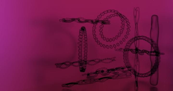


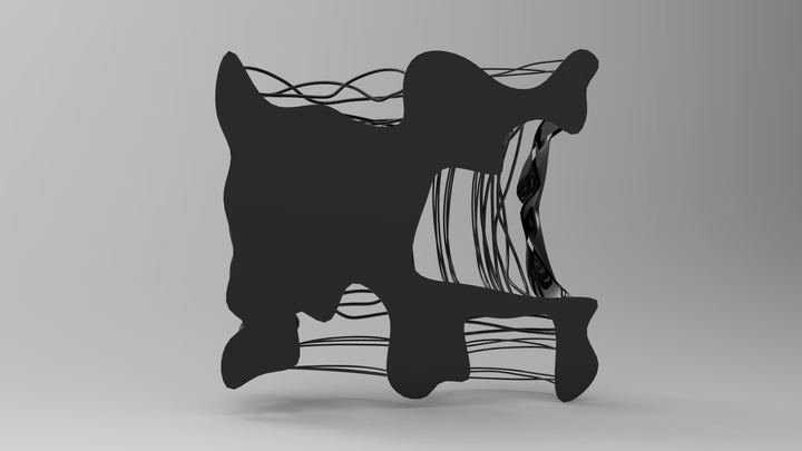


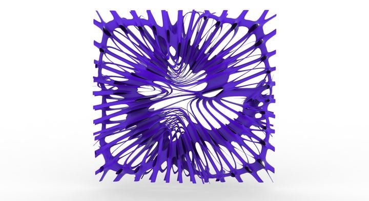
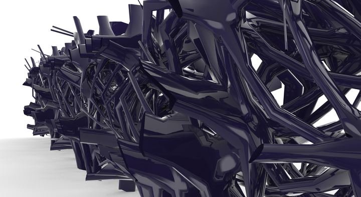
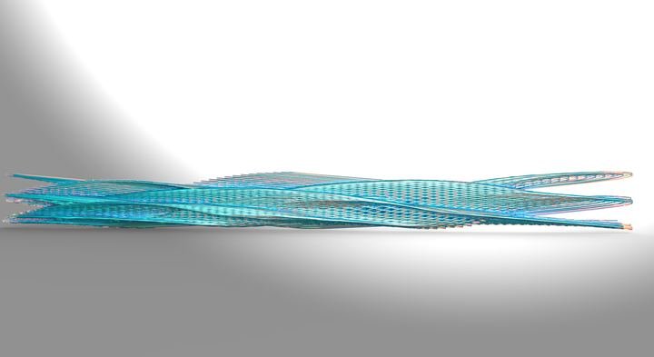


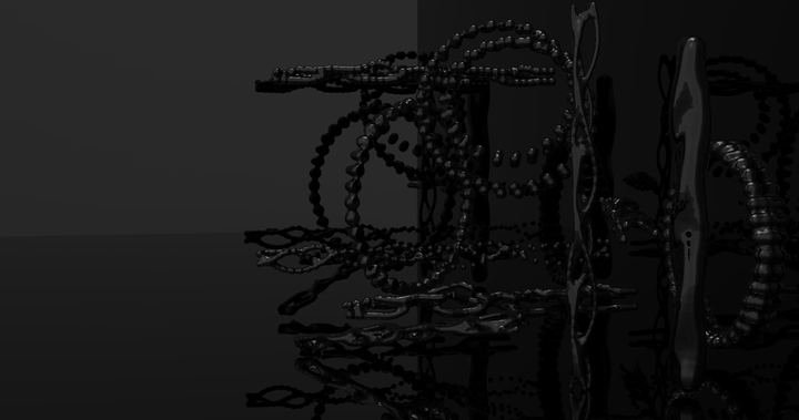

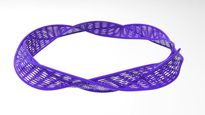
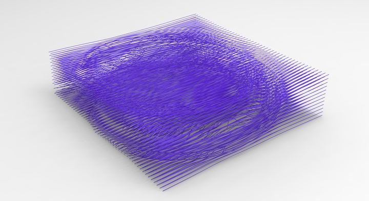
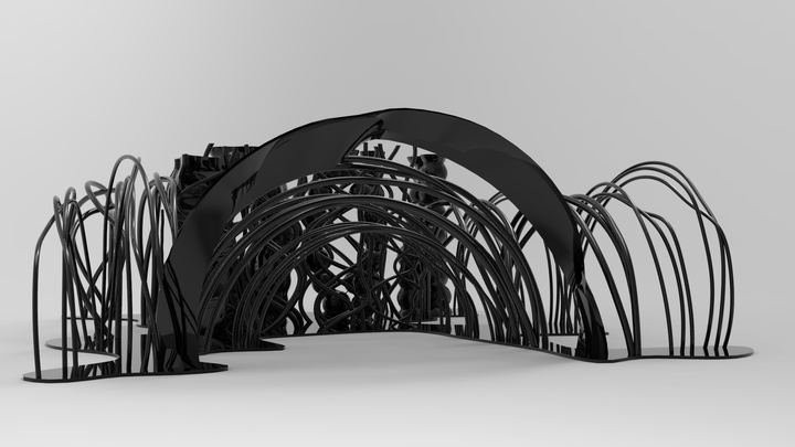
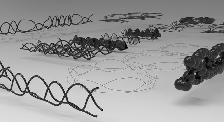

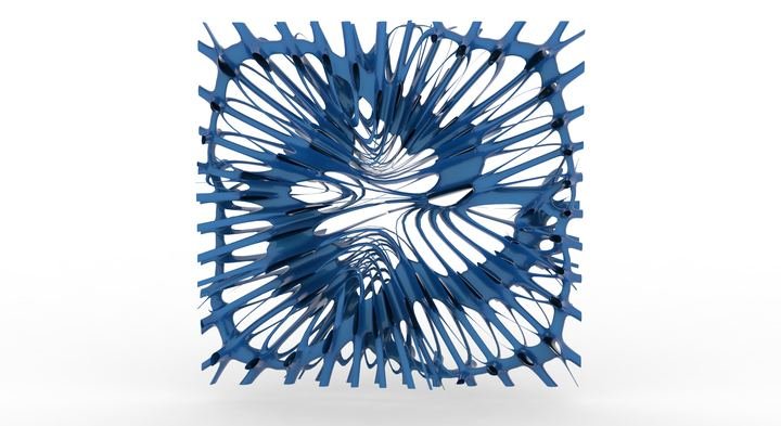


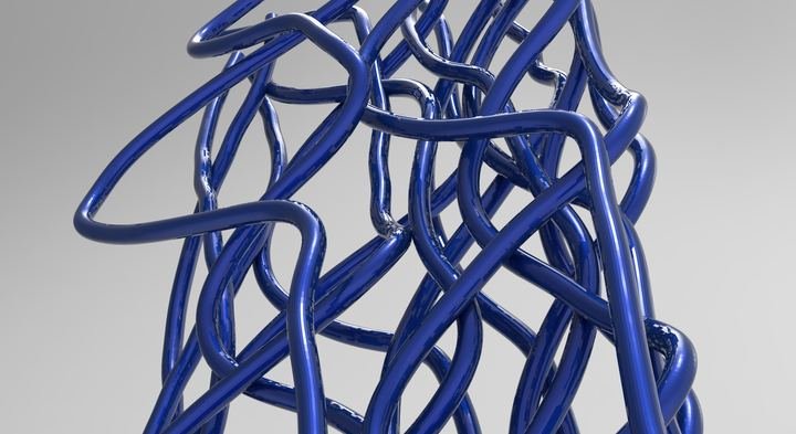


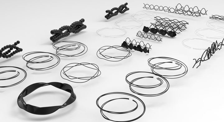
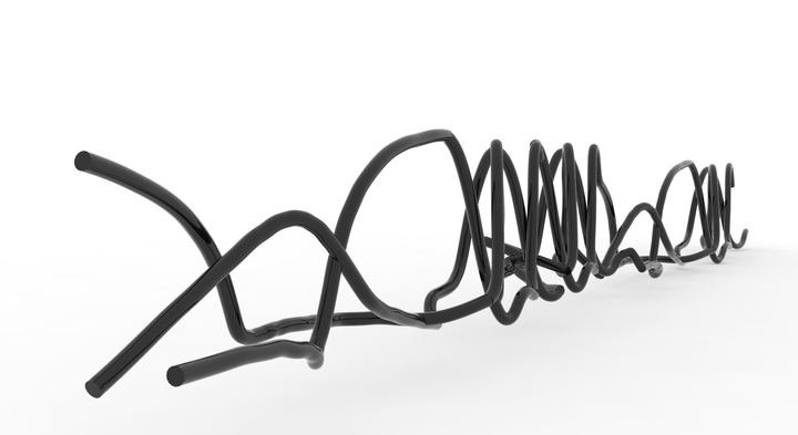

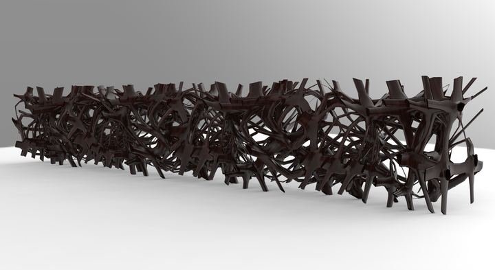

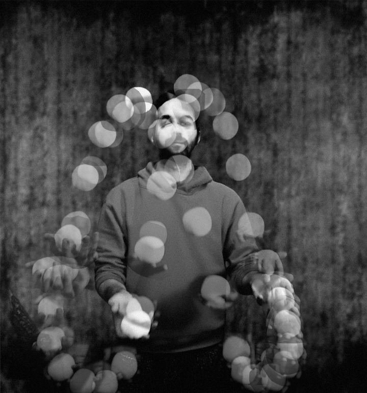

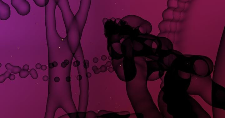

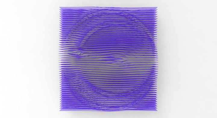
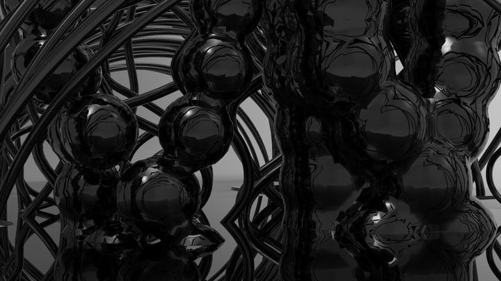


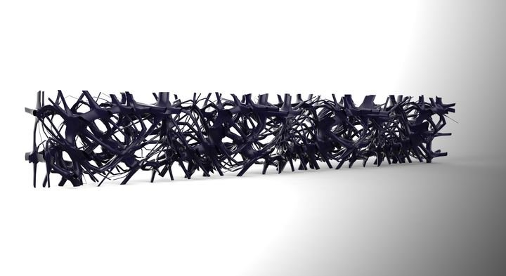


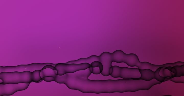


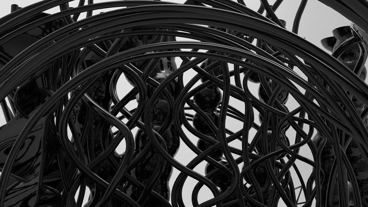

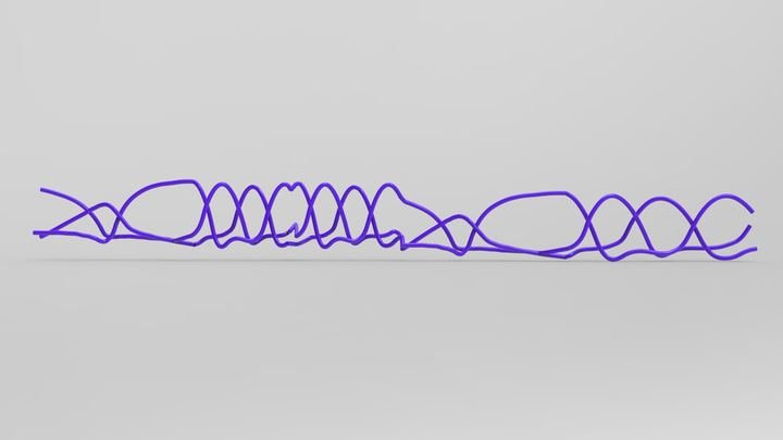


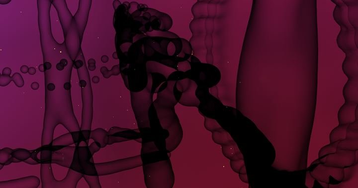

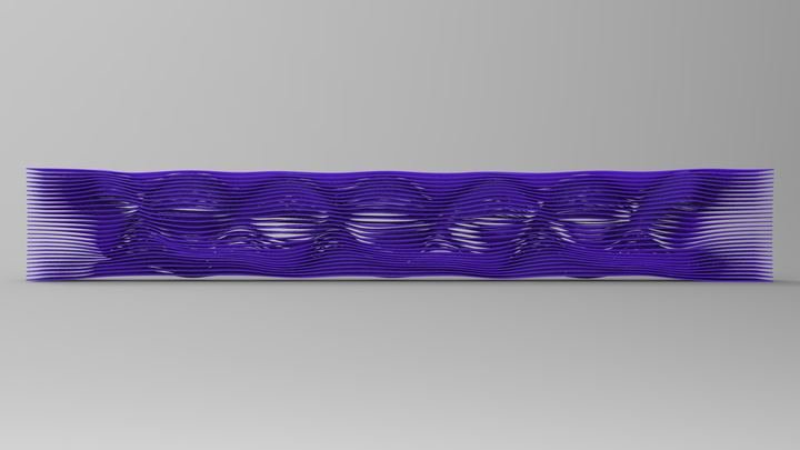
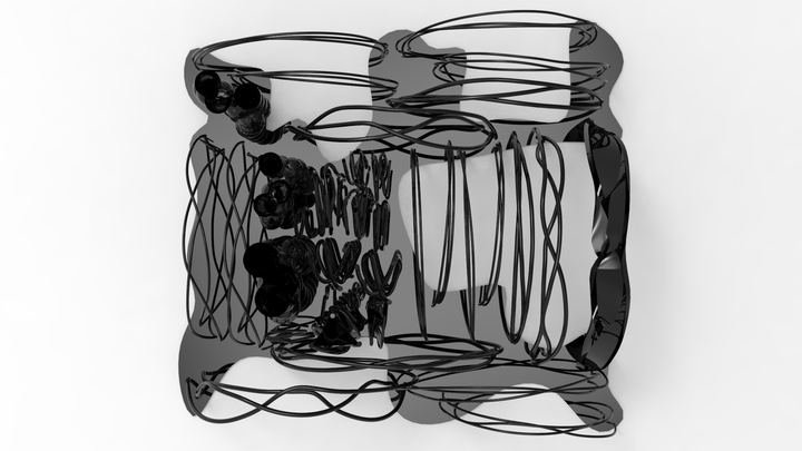


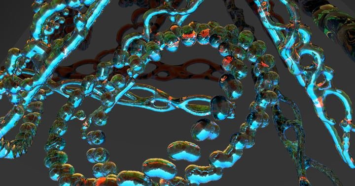
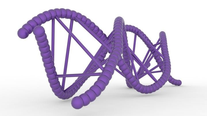


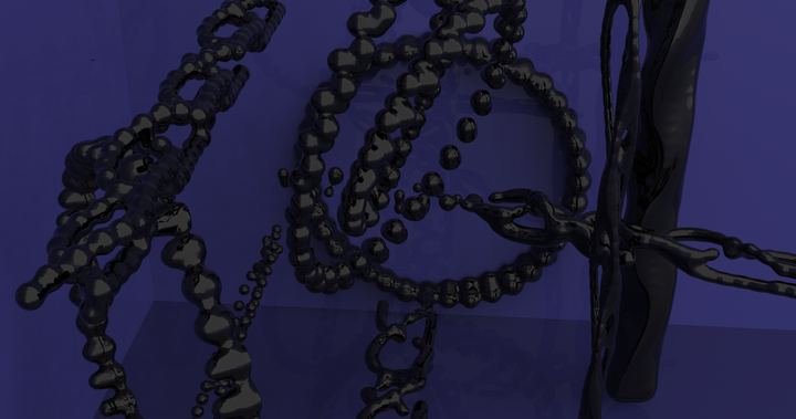


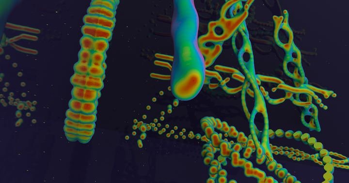





references
Sources cited on this page. The full bibliography of the thesis is included in the thesis text in the research archive.
- Beek, Peter J. and Arthur Lewbel. 1995. “The Science of Juggling.” Scientific American, November 1995: 92–97.
- Bianconi, Fabio, Marco Filippucci and Chiara Verdecchia. 2016. “Body Movement Based Architecture.”
- Buhler, Joe, David Eisenbud, Ron Graham and Colin Wright. 1994. “Juggling Drops and Descents.” The American Mathematical Monthly 101 (6): 507–519.
- Burry, Jane and Mark Burry. 2010. The New Mathematics of Architecture. London: Thames & Hudson.
- Burry, Mark. 2016. “Antoni Gaudí and Frei Otto: Essential Precursors to the Parametricism Manifesto.” Architectural Design 86 (2).
- Coope, Ursula. 2005. Time for Aristotle: Physics IV.10–14. New York: Oxford University Press.
- Einstein, Albert. 1920a. Relativity: The Special and General Theory. Trans. Robert W. Lawson. New York: Henry Holt and Company.
- Einstein, Albert. 1920b. “Time, Space, and Gravitation.” Science 51: 8–10.
- El Sayary, Samer. 2017. “Adding Time Dimension as a Shaping Parameter of Architectural Form (Chrono Form): Fusing Time and Space in Chronoform Wayfinding.” International Journal of Parallel, Emergent and Distributed Systems 32: S26–S38.
- Emmer, Michele. 2016. “Topological Fluid Architecture: Is It Really Architecture?” Xy 1 (1): 68–83.
- Falcon, Andrea. 2013. “Aristotle on Time and Change.” In A Companion to the Philosophy of Time, ed. Adrian Bardon and Heather Dyke, 49–50. Chichester: Wiley-Blackwell.
- Jensenius, Alexander Refsum. 2013. “Some Video Abstraction Techniques for Displaying Body Movement in Analysis and Performance.” Leonardo 46 (1): 53–60.
- Kolarevic, Branko, ed. 2003. Architecture in the Digital Age: Design and Manufacturing. New York and London: Spon Press.
- Lynn, Greg. 1993. “Architectural Curvilinearity: The Folded, the Pliant and the Supple.” Architectural Design 63: Folding in Architecture. Londra: Academy Editions.
- Lynn, Greg. 1998. Folds, Bodies & Blobs: Collected Essays. Brussels: La Lettre Volée.
- Lynn, Greg. 1999a. Animate Form. New York: Princeton Architectural Press.
- Lynn, Greg. 1999b. “Dirim Zaman / Bio Time.” Trans. Özlem Deniz. Mimarlar Derneği 1927 (Association of Architects 1927), no. 5: 275.
- Lynn, Greg. 2005. “Organic Algorithms in Architecture.” TED talk. ted.com
- Marey, Étienne-Jules. 1984. La Chronophotographie. Ed. Michel Frizot. Beaune: Association des Amis de Marey and Ministère de la Culture.
- Massumi, Brian. 2013. “Becoming Affirmative Critique.” Architectural Design 83 (1): 52.
- Motte, Andrew, trans. 1846. Newton’s Principia: The Mathematical Principles of Natural Philosophy. New York: Daniel Adee.
- Özgencil Yıldırım, Sercan. 2017. “A Concept Produced from Design Practice: Sensogram.” 2nd International Congress on Engineering, Architecture and Design, Congress Book: 77–78.
- Piedade Ferreira, M., Duarte Cabral de Mello and José Pinto Duarte. 2011. “The Grammar of Movement: A Step Towards a Corporeal Architecture.” Nexus Network Journal 13 (1): 131–149.
- Schumacher, Michael. 2010. “The Poetics of Movement in Architecture.” In Move: Architecture in Motion – Dynamic Components and Elements, 8. Basel: Birkhäuser.
- Sutil, Nicolás Salazar. 2015. Motion and Representation: The Language of Human Movement. Cambridge, MA: MIT Press.
- Thein, Karel. 2021. “Planets and Time: A Timaean Puzzle.” In Plato’s Timaeus: Proceedings of the Tenth Symposium Platonicum Pragense, 104–107. Leiden: Brill.
- Toulmin, Stephen. 1959. “Criticism in the History of Science: Newton on Absolute Space, Time, and Motion, I.” The Philosophical Review 68 (1).
- Turetzky, Philip. 1998. Time. London and New York: Routledge.
- Vázquez, Daniel. 2022. “Before the Creation of Time in Plato’s Timaeus.” In Time and Cosmology in Plato and the Platonic Tradition, 119.